Scale effects

Idea-based growth models are linked tightly to increasing returns to scale, as was noted earlier in the Idea Diagram. The mechanism at the heart of this link is nonrivalry: the fact that knowledge can be used by an arbitrarily large number of people simultaneously without degradation means that there is something special about the first instantiation of an idea.

Notice that nothing in this argument relies on a low marginal cost of production or on the absence of learning and human capital. Consider the design of a new drug for treating high blood pressure. Discovering the precise chemical formulation for the drug may require hundreds of millions of dollars of research effort. This idea is then simply a chemical formula. Producing copies of the drug - pills - may be expensive, for example if the drug involves the use of a rare chemical compound. It may also be such that only the best-trained biochemists have the knowledge to understand the chemical formula and manufacture the drug. Nevertheless, an accurate characterization of the production technology for producing the drug is as a fixed research cost followed by a constant marginal cost. Once the chemical formula is discovered, to double the production of pills we simply double the number of highly-trained biochemists, build a new (identical) factory, and purchase twice as much of the rare chemical compound used as an input.

Because the link between idea-based growth theory and increasing returns is so strong, the role of “scale effects” in growth models has been the focus of a series of theoretical and empirical papers.

To use an analogy from the computer software industry, are scale effects a bug or a feature? I believe the correct answer is slightly complicated. I will argue that overall they are a feature, i.e. a useful prediction of the model that helps us to understand the world. However, in some papers, most notably in the first generation of idea-based growth models, these scale effects appeared in an especially potent way, producing predictions in these models that are easily falsified. This strong form of scale effects - in which the long-run growth rate of the economy depends on its scale - is a bug. Subsequent research has remedied this problem, maintaining everything that is important about idea­based growth models but eliminating the strong form of the scale effects prediction. This still leaves us, as discussed above, with a weak form of scale effects: the size of the economy affects, in some sense, the level of per capita income. This, of course, is nothing more than a statement that the economy is characterized by increasing returns to scale. The weak form of scale effects has its critics as well, but I will argue two things.

The remainder of this section consists of two basic parts. Section 5.1 returns to the simple growth model presented in Section 3 to formalize the strong and weak versions of scale effects. The remaining sections then discuss a range of applications in the literature related to scale effects.

5.1. Strong and weak scale effects

We could go further and incorporate human capital, as we did in the richer model of Section 4, but this will not change the basic result, so we will leave out this complication.

Now consider two cases. In the first, we impose the condition that φ < 1. In the second, we will instead assume that φ = 1. In the case of φ < 1, the analysis goes through exactly as in the models developed earlier, and the growth rate of the stock of ideas along a balanced growth path is given by

which pins down all the key growth rates in the model. Notice that, as before, the growth rate is proportional to the rate of population growth. It is straightforward to show, as we did earlier, that the level of per capita income in such an economy is an increasing function of the size of the population. That is, this model exhibits weak scale effects. Finally, notice that this equation cannot apply if φ = 1; in that case, the denominator would explode.

To see more clearly the source of the problem, rewrite the idea production function when we assume φ = 1 as

In this case, the growth rate of knowledge is proportional to the number of researchers raised to some power λ.

The first generation idea-based growth models of Romer (1990), Aghion and Howitt (1992) and Grossman and Helpman (1991) all include idea production functions that essentially make the assumption of φ = 1, and all exhibit the strong form of scale effects.^[20] The problem with the strong form of scale effects is easy to document and un­derstand. Because the growth rate of the economy is an increasing function of research effort, these models require research effort to be constant over time to match the relative

stability of growth rates in the United States and some other advanced economies. How­ever, research effort is itself growing over time (for example, if for no other reason than simply because the population is growing). These facts are now documented in more detail.

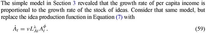
A useful stylized fact that any growth model must come to terms with is the relative stability of growth rates in the United States over more than a century. This stability can be easily seen by plotting per capita GDP for the United States on a logarithmic scale, as shown in Figure 1. A straight line with a growth rate of 1.8 percent per year provides a very accurate description of average growth rates in the United States dating back to 1870. There are departures from this line, of course, most clearly corresponding to the Great Depression and the recovery following World War II. But what is truly remarkable about this figure is how well a straight line describes the trend.

Jones (1995b) made this point in the following way. Suppose one drew a trend line using data from 1870 to 1929 and then extrapolated that line forward to predict per capita GDP today. It turns out that such a prediction matches up very well with the current level of per capita GDP, confirming the hypothesis that growth rates have been relatively stable on average.^[21]

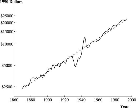
Figure 1.

This stylized fact represents an important benchmark that any growth model must match. Whatever the engine driving long run growth, it must (a) be able to produce relatively stable growth rates for a century or more, and (b) must not predict that growth rates in the United States over this period of time should depart from such a pattern. To see this force of this argument, consider first a theory like Lucas (1988) that predicts that investment in human capital is the key to growth. In this model, the growth rate of the economy is proportional to the investment rate in human capital. But if investment rates in human capital have risen significantly in the 20th century in the United States, as data on educational attainment suggests, this is a problem for the theory. It could be rescued if investment rates in human capital in the form of on-the-job training have fallen to offset the rise in formal education, but there is little evidence suggesting that this is the case.

This stylized fact is even more problematic for the first-generation idea-based growth models of Romer (1990), Aghion and Howitt (1992) and Grossman and Helpman (1991) (R/AH/GH). These models predict that growth is an increasing function of research effort, but research effort has apparently grown tremendously over time. As one example of this fact, consider Figure 2. This figure plots an index of the number of scientists and engineers engaged in research in the G-5 countries. Between 1950 and 1993, this index of research effort rose by more than a factor of eight. In part this is because of the general growth in employment in these countries, but as the figure shows, it also reflects a large increase in the fraction of employment devoted to research. A similar fact can be

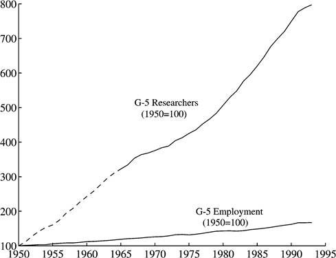
Figure 2. Researchers and employment in the G-5 countries (index). Note.

documented using just the data for the United States, or by looking at spending on R&D rather than employment.^[22] The bottom line is that resources devoted to research have exhibited a tremendous amount of growth in the post-war period, while growth rates in the United States have been relatively stable. The implication is that models that exhibit strong scale effects are inconsistent with the basic trends in aggregate data. Evidence like this is one of the main arguments in favor of models that exhibit weak scale effects instead.^[23]

5.3. Growth effects and policy invariance

At some level, the rejection of models with strong scale effects in favor of models with weak scale effects should not be especially interesting. The only difference between the two models, as discussed above, is essentially the strength of the knowledge spillover parameter. In expanding variety models, is φ = 1 or is φ < 1? Nothing in the evidence necessarily rules out φ = 0.95, and continuity arguments suggest that the economics of φ = 0.95 and φ = 1 cannot be that different.

The main difference in the economic results that one obtains in the two models per­tains to the ability of changes in policy to alter the long-run growth rate of the economy. In the models that exhibit strong scale effects, the long-run growth rate is an increasing function of the number of researchers. Hence, a policy that increases the number of re­searchers, such as an R&D expenditure subsidy, will increase the long-run growth rate. In contrast, if φ < 1, then the long-run growth rate depends on elasticities of produc­tion functions and on the rate of population growth. To the extent that these parameters are unaffected by policy - as one might naturally take to be the case, at least to a first approximation - policy changes such as a subsidy to R&D or a tax on capital will have no affect on the long-run growth rate. They will of course affect the long-run level of income and will affect the growth rate along a transition path, but the long-run growth rate is invariant to standard policy changes.

This statement can be qualified in a couple of ways. First, the population growth rate is really an endogenous variable determined by fertility choices of individuals. Policy changes can affect this choice and hence can affect long-run growth even in a model with weak scale effects, as shown in Jones (2003). However, the effects can often be counter to the usual direction. For example, a subsidy to R&D can lead people to per­form more research and have fewer kids, reducing fertility. Hence a subsidy to research can reduce the long-run growth rate. This can be true even if it is optimal to subsidize research - this kind of model makes clear that long-run growth and welfare are two very different concepts. The second qualification is that one can imagine subsidies that af­fect the direction of research and that can possibly affect long-run growth. For example, Cozzi (1997) constructs a model in which research can proceed in different directions that may involve different knowledge spillover elasticities. By shifting research to the directions with high spillovers, it is possible to change the long-run growth rate.

Despite these qualifications, it remains true that in the semi-endogenous growth mod­els written to address the problem of strong scale effects, straightforward policies do not affect the long-run growth rate. This has led a number of researchers to seek alternative means of eliminating the strong scale effects prediction while maintaining the potency of policy to alter the long-run growth rate. Key papers in this line of research include Young (1998), Peretto (1998), Dinopoulos and Thompson (1998) and Howitt (1999) (Y/P/DT/H).

These papers all work in a similar way.²⁴ In particular, each adds a second dimension to the model, so that research can improve productivity for a particular product or can add to the variety of products. To do this in the simplest way, suppose that aggregate consumption (or output) is a CES composite of a variety of different products

where B_t represents the variety of goods that are available at date t and Y_it is the output of variety i. Assume that each variety Y_i is produced using the Romer-style technology with φ — 1 in the simple model given earlier in Section 3.

The key to the model is the way in which the number of different varieties B changes over time. To keep the model as simple as possible, assume

That is, the number of varieties is proportional to the population raised to some power β. Notice that this relationship could be given microfoundations with an idea production function analogous to that in Equation (16).²⁵

Finally, let us assume each intermediate variety is used in the same quantity so that Y_it — Y_t, implying C_t — Bf Y_t. Per capita consumption is then c_t — Bfy_t, and per capita consumption growth along a balanced growth path is

Assuming an idea production function with φ — 1, like that in R/AH/GH, the growth rate of the stock of ideas is proportional to research effort per variety, LA_t∕B_t — sL_t∕B_t,

^[1] This section draws heavily on Jones (1999).

^[1] For example, if B — LB^γ, then Equation (63) holds along a balanced growth path with β — 1/(1 — γ).

Substituting this equation back into (64) gives the growth rate of per capita output as a function of exogenous variables and parameters

With β = 1 so that B_t = L_t, the strong scale effect is eliminated from the model, while the effect of policy on long-run growth is preserved. That is, a permanent increase in the fraction of the labor force working in research, ₁s^,, will permanently raise the growth rate. This is the key result sought by the Y/P/DT/H models.

However, there are two important things to note about this result. First, it is very frag­ile. In particular, to the extent that β = 1, problems reemerge. If β < 1, then the model once again exhibits strong scale effects. Alternatively, if β > 1, then changes in ∙s∙ no longer permanently affect the long-run growth rate. Thus, the Y/P/DT/H result depends crucially on a knife-edge case for this parameter value, in addition to the Romer-like knife-edge assumption of φ = 1. Second, as the first term in Equation (66) indicates, the model still exhibits the weak form of scale effects. This result is not surprising given that these are idea-based growth models, but it is useful to recognize since many of the papers in this literature have titles that include the phrase “growth without scale effects”. What these titles really mean is that the papers attempt to eliminate strong scale effects; all of them still possess weak scale effects. These points are discussed in more detail in Jones (1999) and Li (2000, 2002).

5.3. Cross-country evidence on scale effects

One source of evidence on the empirical relevance of scale effects comes from looking across countries or regions at a point in time. Consider first the ideal cross-sectional evidence. One would observe two regions, one larger than the other, that are otherwise identical. The two regions would not interact in any way and the only source of new ideas in the two regions would be the regions’ own populations. In such an ideal ex­periment, one could search for scale effects by looking at the stock of ideas and at per capita income in each region over time. In the long-run, one would expect that the larger region would end up being richer.

In practice, of course, this ideal experiment is never observed. Instead, we have data on different countries and regions in the world, but these regions almost certainly share ideas and they almost certainly are not equal in other dimensions. It falls to clever econo­metricians to use this data to approximate the ideal experiment. No individual piece of evidence is especially compelling, but the collection taken together does indeed suggest that the cross-sectional evidence on scale effects supports the basic model.

Certainly the most creative approximation to date is found in Kremer (1993) and later appears in the Pulitzer Prize-winning book Guns, Germs, and Steel by Diamond (1997). The most recent ice age ended about 10,000 B.C. Before that time, ocean levels were lower, allowing humans to migrate around the world - for example across the Bering Strait and into the Americas. In this sense, ideas could diffuse across regions. However,

with the end of the ice age, sea levels rose, and various regions of the world were effec­tively isolated from each other, at least until the advent of large sailing ships sometime around the year 1000 or 1500. In particular, for approximately 12,000 years, five regions were mutually isolated from one another: the Eurasian/African continents, the Ameri­cas, Australia, Tasmania (an island off the coast of Australia), and the Flinders Island (a very small island off the coast of Tasmania). These regions are also nicely ranked in terms of population sizes, from the relatively highly-populated Eurasian/African conti­nent down to the small Flinders Island, with a population that likely numbered fewer than 500.

It is plausible that 12,000 years ago these regions all had similar technologies: all were relatively primitive hunter-gatherer cultures. Now fast-forward to the year 1500 when a wave of European exploration reintegrates the world. First, the populous Old World has the highest level of technological sophistication; they are the ones doing the exploring. The Americas follow next, with cities, agriculture, and the Aztec and Mayan civilizations. Australia is in the intermediate position, having developed the boomerang, the atlatl, fire-making, and sophisticated stone tools, but still consisting of a hunter­gatherer culture. Tasmania is relatively unchanged, and the population of Flinders Island had died out completely. The technological rank of these regions more than 10,000 years later matches up exactly with their initial population ranks at the end of the last ice age.

Turning to more standard evidence from the second-half of the 20th century, one is first struck by the apparent lack of support for the hypothesis of weak scale effects. The most populous countries of the world, China and India, are among the poorest, while some of the smallest countries like Hong Kong and Luxembourg are among the richest. And the countries with the most rapid rates of population growth - many in Africa - are among the countries with the slowest rates of per capita income growth. However, a moment’s thought suggests that one must be careful in interpreting this evi­dence. It is clearly not the case that Hong Kong and Luxembourg are isolated countries that grow solely based on the ideas created by their own populations. These countries benefit tremendously from ideas created around the world. And in the case of the poor countries of the world, “other things” are clearly not equal. These countries have very different levels of human capital and different policies, institutions, and property rights that contribute to their poverty. Hence, we must turn to econometric evidence that seeks to neutralize these differences.

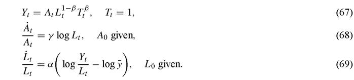
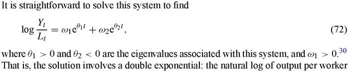
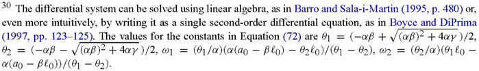
The clearest cross-country evidence in favor of weak scale effects comes from papers that explicitly control for differences in international trade. Intuitively, openness to in­ternational trade is likely related to openness to idea flows, and the flow of ideas from other countries is one of the key factors that needs to be neutralized. Backus, Kehoe and Kehoe (1992), Frankel and Romer (1999) and Alcala and Ciccone (2002) are the main examples of this line of work, and all find an important role for scale. Alcala and Ciccone (2002) provide what is probably the best specification, controlling for both trade and institutional quality (and instrumenting for these endogenous variables), but the results in Frankel and Romer (1999) are similar. Alcala and Ciccone find a long- run elasticity of GDP per worker with respect to the size of the workforce that is equal to 0.20.26 That is, holding other things equal, a 10 percent increase in the size of the workforce in the long run is associated with a 2 percent higher GDP per worker.^{[24] [25]}

Other cross-country studies, of course, have not been able to precisely estimate this elasticity. Hall and Jones (1999), for example, found a point estimate of about 0.05, but with a standard error of 0.06. Sala-i-Martin (1997) does not find the size of the population to be a robust variable in his four million permutations of cross-country growth regressions. Finally, it should be recognized that this cross-country estimate of the scale elasticity is not necessarily an estimate of the structural parameter γ in the idea models presented earlier in Section 4. One needs a theory of technology adoption and idea flows in order to make sense of the estimates. For example, in a world where ideas flow to all places instantaneously, there would be no reason to find a scale effect in the cross-section evidence.

A final piece of evidence that is often misinterpreted as providing evidence against the weak scale effects prediction is the negative coefficient on population growth in a cross-country growth regression, such as in Mankiw, Romer and Weil (1992). Recall that the standard interpretation of these regressions is that they are estimating transition dynamics. The negative coefficient on population growth is interpreted as capturing the dilution of the investment rate associated with the Solow model. Consider two countries that are identical but for different population growth rates. The country with the faster population growth rate must equip a larger number of new workers with the existing capital-labor ratio, effectively diluting the investment rate. The result is that such an economy has a lower capital-output ratio in steady state, reducing output per worker along the balanced growth path. But this same force is also at work in any growth model, including idea-based models, as was apparent above in Result 1(b). The implication is that this cross-country evidence is not inconsistent with models in which weak scale effects play a role.

5.4. Growthovertheverylongrun

Additional evidence on the potential relevance of scale effects to economic growth comes from what at first might seem an unlikely place: the history of growth from thousands of years ago to the present.

One of the important applications of models of economic growth in recent years has been to understand economic growth over this very long time period. Many of our workhorse models of growth were constructed with an eye toward 20th-century growth. Asking how well they explain growth over a much longer period of time therefore pro­vides a nice test of our models.

Figure 3. World per capita GDP (log scale). Note. Data from Maddison (1995) for years after 1500. Before 1500, we assume a zero growth rate, as suggested by Maddison and others.

The key fact that must be explained over this period is quite stunning and is displayed in Figure 3. For thousands and thousands of years prior to the Industrial Revolution, standards of living were relatively low. In particular, the evidence suggests that there was no sustained growth in per capita incomes before the Industrial Revolution.^[26] Then, quite suddenly from the standpoint of the sweep of world history, growth rates accel­erated and standards of living began rising with increasing rapidity. At the world level, per capita income today is probably about 10 times higher than it was in the year 1800 or 1500 or even 10,000 years ago. A profound question in economic history - and one that growth economists have begun delving into - is this: How do we understand this entire time path? Why were standards of living relatively low and stagnant for so long, why have they risen so dramatically in the last 150 years, and what changed?^[27]

The recent growth literature on this question is quite large, and a thorough review is beyond the scope of the present chapter (additional discussion can be found in Chapter 4 of this Handbook, by Oded Galor). Representative papers include Lee (1988), Kremer (1993), Goodfriend and McDermott (1995), Lucas (1998), Galor and Weil (2000), Clark (2001), Jones (2001), Stokey (2001), Hansen and Prescott (2002) and Tamura (2002).

In several of these papers, scale effects play a crucial role. Scale is at the heart of the models of Lee (1988), Kremer (1993) and Jones (2001), and it also plays an important role in getting growth started in the model based on human capital in Galor and Weil (2000).

The role of scale effects in these models can be illustrated most effectively by looking at the elegant model of Lee (1988). The three key equations of that model are:

Equation (67) describes a production function that depends on ideas A, labor L, and land T, which is assumed to be in fixed supply and normalized to one. Equation (68) is a Romer-like production function for new ideas. Notice that we have assumed the φ = 1 case so that we can get an analytic solution below, but the nature of the results does not depend on this assumption. Notice also that we assume all labor can produce ideas, and we assume a log form. This makes the model log-linear, which is the sec­ond key assumption needed to get a closed-form solution. Finally, Equation (69) is a Malthusian equation describing population growth. If output per person is greater than the subsistence parameter y, then population grows; if less then population declines.

The model can be solved as follows. First, choose the units of output such that the subsistence term gets normalized to zero, log y = 0. Next, let a ? log A and I ? log L. Then the model reduces to a linear homogeneous system of differential equations:

grows exponentially, so that the growth rate of output per worker, y ? Y/L, itself grows exponentially,

Mathematically, it is this double exponential growth that allows the model to deliver a graph that looks approximately like that in Figure 3.

Analytically, Lee’s result is extremely nice. However, the analytic results are obtained only by simplifying the model considerably - perhaps too much. For example, the model generates double exponential growth in population as well. As shown in Kremer (1993), this pattern fits the broad sweep of world history, but it sharply contradicts the demo­graphic transition that has set in over the last century, where population growth rates level off and decline. In addition, the analytic results require the strong assumption that Φ = 1.

If one wishes to depart from the log-linear structure of Lee’s model, the analysis must be conducted numerically. This is done in Jones (2001), with a more realistic demographic setup and with an idea production function that incorporates φ < 1. The basic insights from Lee (1988) apply over the broad course of history, but the model also predicts a demographic transition and a leveling off of per capita income growth in the 20th century. The model with weak scale effects, then, is able to match the basic facts of income and population growth over both the very long run and the 20th century.

The economic intuition for these results is straightforward. Thousands and thousands of years ago, the population was relatively small and the productivity of the population at producing ideas was relatively low. Per capita consumption, then, stayed around the Malthusian level that kept population constant (y in the Lee model above). Suppose it took 1000 years for this population to discover a new idea. With the arrival of the new idea, per capita income and fertility rose, producing a larger population. Diminishing returns associated with a fixed supply of land drove consumption back to its subsistence level, but now the population was larger. Instead of requiring 1000 years to produce a new idea, this larger population produced a new idea sooner, say in 800 years. Con­tinuing along this virtuous circle, growth gradually accelerated. Provided the economic environment is characterized by a sufficiently large degree of increasing returns (to off­set the diminishing returns associated with limited land), the acceleration in population growth produces a scale effect that leads to the acceleration of per capita income growth. Eventually, the economy becomes sufficiently rich that a demographic transition sets in, leading population growth and per capita income growth to level out.^[28]

5.5. Summary: scale effects

Virtually all idea-based growth models involve some kind of scale effect, for the basic reason laid out earlier in the presentation of the Idea Diagram. The strong scale effects of many first-generation idea-based growth models - in which the growth rate of the economy is an increasing function of its size - are inconsistent with the relative stability of growth rates in the United States in the 20th century. Subsequent idea-based growth models replaced this strong scale effect with a weak scale effect, where the long-run level of per capita income is an increasing function of the size of the economy. The long-run growth rate in these models is generally an increasing function of the rate of growth of research effort, which in turn depends on the population growth rate of the countries contributing to world research. However, this growth rate is typically taken to be exogenous, producing the policy-invariance results common in these models.

Simple correlations (say of income per person with population, or growth rates of per capita income with population growth rates) on first glance appear to be inconsistent with weak scale effects. However, the ceteris paribus assumption is not valid for such comparisons. Attempts to render other things equal using careful econometrics certainly reveal no inconsistency with the weak scale effects prediction, although they also do not necessarily provide precise estimates of the magnitude of the key scale elasticity.

More broadly, the very long-run history of economic growth appears consistent with weak scale effects. Models in which scale plays an important role have proven capable of explaining the very long-run dynamics of population and per capita income, includ­ing the extraordinarily slow growth over much of history and the transition to modern economic growth since the Industrial Revolution.

6.