4.2 Thedynamics
As in the previous chapter, we can treat the entrepreneurs' wealth WB as the state variable. In fact, in an open economy the dynamics is simpler than in a closed economy in the sense that we do not need to keep track of domestic aggregate savings, and therefore of the wealth of domestic lenders.
The reason is that loans come from both, domestic and foreign lenders and the total amount of loanable funds is therefore always greater than the investment capacity μWj, of domestic borrowers. Actual investment is thus always constrained by the wealth constraints of domestic firms, never by the supply of funds. We first derive the dynamic equations that describe the evolution of entrepreneurs' wealth over time. We then show under which conditions the open economy converges to a limit cycle.4.2.1 Dynamicequations 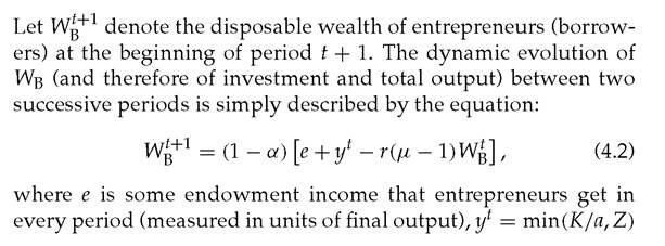
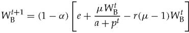
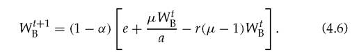
is output in period t (also equal to the gross revenues of entrepreneurs during that period). The expression in brackets is the net end-of-period t revenue of entrepreneurs. The net disposable wealth of entrepreneurs at the beginning of period t + 1 is what remains of this net end-of-period return after consumption, hence the multiplying factor (1 — α) on the right-hand side of equation (4.2).
Entrepreneurs invest and borrow only if their profits are larger than or equal to the international return. When μ or Wb are large, entrepreneurs invest only up to the point where y — rL = vWb, where L denotes the amount of borrowings. Any remaining wealth is invested at the international market rate. In this case, no pure profits are earned from production and the evolution of wealth is simply given by:
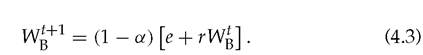
Thus, the dynamics are fully described either by difference equation (4.2) or by difference equation (4.3) and we now proceed to analyze under which conditions this dynamic system generates persistent endogenous fluctuations.
4.2.2 Two main effects of current wealth on future wealth
Let It = μWB denote the borrowing (or investment) capacity of domestic entrepreneurs at the beginning of period t + 1. Entrepreneurs will choose the level of the country-specific factor z, with corresponding investment Kt = It — pt ∙ z, to maximize current profits, where pt still denotes the current price of the nontradable (or country-specific) good in terms of the tradable. Given the above Leontief technology, the optimum involves
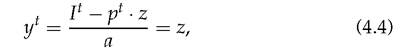
which in turn yields
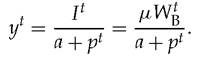
The dynamic equation (4.2) can thus be rewritten:

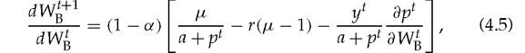
which in turn reveals two opposite effects of current wealth on future wealth.
1. A wealth effect. This effect corresponds to the term (μ∕(a + pt) — r(μ — 1)) on the right-hand side of (4.3). In other words: for given price of the nontradable good, a higher level of current wealth WB leads to higher output, which in turn improves the creditworthiness of entrepreneurs and thereby generates greater investment demand over the next period. This effect generates investment booms and a positive effect of current wealth on future wealth.
2. A price effect. This effect is captured by the term yt∕(a + pt) ? ∂pt ∕∂ WB on the right-hand side of (4.3). In other words, higher wealth in this period increases entrepreneurs' investment demand, and therefore the demand for the nontradable input.
As a result, the price of that input—pt—increases, which in turn reduces entrepreneurs' borrowing capacity next period, and therefore their output and wealth. Whenever it dominates, this effect will carry the economy from a boom to a slump.We now show how the combination of these two effects may result in persistent fluctuations, and how the booms and slumps
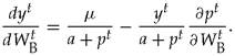
2 Here we use the fact that:
in these fluctuations share many features with those observed in practice.
4.2.3 Existence of limit cycles
Figure 4.1 depicts future wealth as a function of current wealth as implied by the dynamic equation (4.3) in the Leontief case. As one can see, the curve consists of three pieces, corresponding respectively to low, intermediate, and high levels of current wealth. Let us look at those three regions in more details.
Suppose first that current wealth W1B is sufficiently small that the credit constraint is binding (L = (μ — 1)WB) and entrepreneurs do not have enough wealth to use the whole endowment of nontradable input under the Leontieftechnology ((μWB/a) < Z). In this case, there is an excess supply of the nontradable input. This immediately yields: pt = 0. Output at date t is then given by: 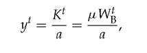
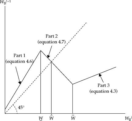
Fig. 4.1 Phase diagram with Leontief technology.
Source: Aghion et al. (2004a), figure 1.
so that
This equation corresponds to the first piece in Figure 4.1. Here no price effect is at work. There is only a wealth effect, and this is why an increase in current wealth leads unambiguously to an increase in future wealth.
Now, suppose that current wealth WB remains sufficiently small that the credit constraint is still binding (L = (μ — 1)W^), but that entrepreneurs now have enough wealth, and therefore enough investment capacity, to exhaust the whole supply of nontradable input under the Leontief technology (i.e.
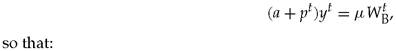
(Kt∕a) ≥ Z). Thus, there is excess demand for the immobile factor. In that case, the equilibrium price pt of the nontradable input becomes positive, and output is determined in equilibrium by the aggregate supply of that input: yt = Z. From (4.4) and the definition of I, the equilibrium price of the country-specific input is given by: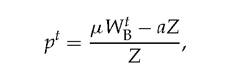
so that future wealth is now determined by the dynamic equation: 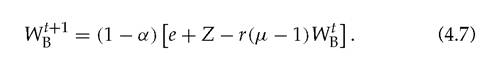 This equation corresponds to the second piece in Figure 4.1. There, only the price effect is at work (since output is fixed at yt = Z), which explains why this branch is downward sloping.
Finally, when current wealth WB is sufficiently large enough that entrepreneurs are no longer credit constrained (i.e. L < (μ — 1)W^), then as in the previous case the equilibrium price of the nontradable input pt is positive and output remains fixed at yt = Z, but the price pt is no longer affected by the level of investment. When WB is that large, entrepreneurs will borrow until profits equal the international interest rate. In other words, they are indifferent between lending on the international market or investing in their own project, which in turn yields the dynamic equation (4.3). This equation corresponds to the third, again upward sloping, piece in Figure 4.1.
As drawn in Figure 4.1, the 45o line intersects the W^+1 (W^) curve at the point W which lies in the second segment. This intersection can also be in either of the other two segments. It will be in the first segment when (1 — α)e∕(1 — (1 — α){(μ∕a) — r(μ — 1)}), the fixed point of equation (4.6), is less than W = aZ∕μ. Since (1 — α)e∕(1 — (1 — α){(μ∕a) — r(μ — 1)}) is increasing in μ while W is decreasing, it is clear that this can only happen when μ is very small.
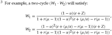
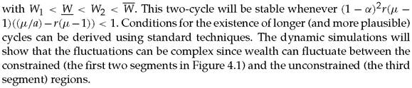
On the other hand, the intersection will be in the third segment when the fixed point of equation (4.3), (1 — α)e∕(1 — (1 — α)r) > W = Z∕μr. This will only happen when μ is sufficiently large. For intermediate values of μ, corresponding to an intermediate level of financial development, the case is depicted in Figure 4.1. This is the one case where the economy does not converge monotonically to its steady state.In this case there are two possibilities—short-run fluctuations, represented by oscillations that eventually converge to the steady state, W, and long-run volatility, represented by a system which does not converge to a steady state but instead continues to oscillate forever. A necessary condition for the existence of such a limit cycle is that the steady state at W be unstable, true only when the slope of the W^+1(W^) schedule at W is less than —1, corresponding to when W lies in the second segment of that schedule. Thus, for long-run volatility to occur, we must have W < W < W and —(1 — α)(μ — 1)r < —1. If these conditions hold, one can easily derive additional sufficient conditions under which long-run volatility actually occurs. 3
Intuitively, the basic mechanism underlying this cyclicality can be described as follows: during a boom the demand for the domestic country-specific factor goes up as (high-yield) investments increase, thus raising its price. This higher price will eventually squeeze investors' borrowing capacity and therefore the demand for country-specific factors. At this point, the economy experiences a slump and two things occur: the relative price of the domestic factor collapses, while a fraction of the factor available remains unused since there is not enough investment.
The collapse in the factor price thus corresponds to a contraction of real output. Of course, the low factor price will eventually lead to higher profits and therefore to more investment. A new boom then begins.[11]The reason why the level of financial development matters is also quite intuitive: economies at a low level of financial development have low levels of investment and do not generate enough demand to push up the price of the country-specific factor while economies at a very high level of development have sufficient demand for that factor to keep its price always positive. It is then at intermediate levels of financial development that shocks to cash flow will have an effect intense enough to be a source of instability.
This last argument also helps us understand why opening the economy to foreign capital may destabilize: essentially, the response of an economy with a closed capital market to a cash flow shock is limited since only so much capital is available to entrepreneurs. Additional funding sources in an open economy potentially increase the response to a shock and therefore the scope for volatility.
4.3
More on the topic 4.2 Thedynamics:
- 4.2 Thedynamics
- Dynamic equations
- Aghion P., Banerjee A.. Volatility and Growth. Oxford, Oxford University Press,2005. - 159p., 2005
- Financial liberalization and instability
- Contents
- Functional forms for the model components
- The convergence hypothesis
- Skill-biased technical change: Inside the black box
- Examples of non-standard questions and outcomes
- Anti-system and Specialized Social Movements