HOW REAL ARE THE NUMBERS?
Many individuals are attracted to business careers not only by monetary rewards but by the opportunity, lacking in many other professions, to be measured against an objective standard.
The personal desire to improve the bottom line, that is, a company’s net profit, challenges a businessperson in much the same way that an athlete is motivated by the quantifiable goal of breaking a world record. The income statement is the stopwatch against which a company runs; net profit is the corporation’s record of wins and losses for the season.The analogy between business and athletics extends to the fact, which is apparent to any close observer, that superior skills and teamwork alone do not win championships. A baseball manager can intimidate the umpire by heatedly protesting a call on the basepaths, hoping thereby to have the next close ruling go in his team’s favor. A corporation has the power to fire its auditor, and may use that power to influence accounting decisions that are matters of judgment, rather than clear-cut reporting standards. A baseball team’s front office can shorten the right-field fence in its home stadium to favor a lineup stocked with left-handed power hitters; a corporation’s management can select the accounting method that shows its results in the most favorable light. Collectively, the team owners can urge the Rules Committee to lower the pitching mound if they believe that a predictable increase in base hits and runs will boost attendance. Similarly, a group of corporations can try to block the introduction of new accounting standards that might reduce their reported earnings.
Attempts to transform the yardstick become most vigorous when the measure of achievement becomes more important to participants than the accuracy of the measure itself.
Regrettably, this is often the case when corporations seek to motivate managers by linking their compensation to the attainment of specific financial goals. Executives whose bonuses rise in tandem with earnings per share have a strong incentive not only to generate bona fide earnings, but also to use every lawful means of inflating the figures through accounting sleight of hand.It would take many more pages than are allotted to this chapter to detail all the ways that companies can manipulate the accounting rules to inflate their earnings. Instead, the following examples should convey to the reader the thought process involved in this rule bending. Equipped with an understanding of how the rule benders think, users of financial statements will be able to detect other ruses they are sure to encounter.
Not All Sales Are Final
“Take care of the top line and the bottom line will take care of itself.” So goes a business bromide, which underscores the importance of revenues (the top line) to net income (the bottom line). The point is that if a company wants to cure an earnings problem, it should concentrate on bringing in more sales.
Generally, this is sound advice, as long as the needed sales are brought in by the salesforce. A company can compound its problems, however, if the financial staff makes up the shortfall in revenues through accounting gimmicks. Some revenue-inflating tricks are achievable within GAAP boundaries, whereas others clearly fall outside the law. They all produce similar ill effects, however. Enhancements to reported sales boost reported earnings without increasing cash flow commensurately.
style='text-indent:18.0pt'>Often, a company’s earnings and cash flow diverge to an extent that becomes unsustainable. The eventual result is an abrupt adjustment to the financial statements of previous periods. In the process, earnings and cash flow come back into alignment, but management’s credibility plummets. Even when no such shock occurs, the practice of pumping up revenues through discretionary accounting decisions represents a hazard for analysts. At a minimum, it reduces the comparability of a company’s financial statements from one period to the next.The revenue recognition practices of International Business Machines came in for criticism when competition heated up in the computer business during the late 1980s. Management responded by becoming more accommodating in its marketing practices. The company stretched out payment periods, offered to make partial refunds if prices were subsequently reduced, and allowed customers to try out equipment without making any initial payments. For additional variations on the theme of aggressive revenue recognition, see Chapter 6.
Additional Reasons to Be Skeptical about Revenues
Unfortunately for analysts, companies do not always spell out in the Notes to Financial Statements the means by which they have artificially inflated their revenues. A company might lower the credit standards it applies to prospective customers without simultaneously raising the percentage of reserves it establishes for losses on receivables. The result would be a rise in both revenues and earnings, in the current p eriod, with the corresponding increase in credit losses not becoming apparent until a later period. Alternatively, a manufacturer may institute short-term discounts that encourage its dealers or wholesalers to place orders earlier than they otherwise would. In this case, sales and earnings will be higher in the current quarter than they would be in the absence of the incentives, but the difference will represent merely a shifting of revenues from a later to an earlier period. Analysts will face disappointment if they regard such inflated quarterly sales as indicative of the future.
Although the current-period income statement may offer no clues that these gambits have been used, several techniques can help the analyst detect artificial expansion of revenues.
On a retrospective basis, a surge in credit losses or an unexpected shortfall in revenues may indicate that revenues were inflated in an earlier period with the techniques described in the preceding paragraph. (Hindsight of this kind is not without value; an analyst who finds a historical pattern of hyperbolized sales will be appropriately skeptical about future income statements that look surprisingly strong.) On a current basis, analysts should take notice if a company posts a substantially greater sales increase than its competitors. If discussions with the company and other industry sources fail to elicit a satisfactory explanation (such as the introduction of a successful new product), artificial methods may be the root of the matter. Industry sources can also provide direct testimony about tactics being used to shift revenues from future periods to the present.Making the Most of Depreciation and Amortization
Along with provisions for credit losses, another major expense category that can be controlled through assumptions is depreciation. As a check against possible abuses, analysts should compare a company’s ratio of depreciation to property, plant, and equipment with the ratios of its industry peers. An unusually low ratio may indicate that management is being unrealistic in acknowledging the pace of wear and tear on fixed assets. Understatement of expenses and overstatement of earnings would result.
Knowing that astute analysts will compare their depreciation policies with competitors’ practices, companies commonly represent accounting changes in this area as efforts to get into line with industry norms. They do not ordinarily stress another plausible motive, a desire to pump up earnings. Verbs such as extend and liberalize are considered expendable in the press releases disclosing revisions in depreciable lives.
Depreciation Assumptions—Fort Howard and Weirton Steel Fort Howard produced a typical announcement of a change in depreciation assumptions in April 1992:
During the first quarter of 1992, the company prospectively changed its estimates of the depreciable lives of certain machinery and equipment.
These changes were made to better reflect the estimated periods during which such assets will remain in service. As a result, the lives over which the company depreciates the cost of its operating equipment and other capital assets will more closely approximate industry norms. For the three months ended March 31, 1992, the change had the effect of reducing depreciation expense by $9.9 million and reducing net loss by $6.1 million.In the same month, Weirton Steel described a change in accounting for depreciation even more tersely. The company did not alter the depreciable lives of the assets, but instead switched its accounting method:
Weirton reported a change in depreciation method (accounting principle) effective January 1, 1992, for its steelmaking facilities from the straight-line method to a production-variable method, which adjusts straight-line depreciation to reflect production levels.
In explaining the change, the company did not emphasize a yearning for conformity with its fellow steelmakers. Nevertheless, Weirton was not the first in its group to abandon straight-line depreciation (already a less conservative technique than the various accelerated methods), for the still more liberal production-variable approach. During the first quarter of 1992, Weirton’s switch in depreciation accounting had the convenient effect of reducing its net loss by nearly half.
A method that “adjusts straight-line depreciation to reflect production levels” may sound innocuous. Analysts should keep in mind, however, that the adjustment is far more likely to be downward than upward. As demand falls, the plant will incur more idle time and the company will record less depreciation expense. The same will be true if the facility turns unprofitable and temporarily shuts down, while lower-cost, more technologically advanced facilities owned by competitors continue to operate.
Under these conditions, the book value of the plant will decline more slowly, even as approaching obsolescence.Extraordinary and Nonrecurring Items
To most individuals who examine a company’s income statement, the document is less important for what it tells about the past than for what it implies about future years.2 Last year’s earnings, for example, have no direct impact on a company’s stock price, which represents a discounting of a future stream of earnings (see Chapter 14). An equity investor is therefore interested in a company’s income statement from the preceding year primarily as a basis for forecasting future earnings. Similarly, a company’s creditors already know whether they were paid the interest that came due in the previous year before the income statement arrives. Their motivation for studying the document is to form an opinion about the likelihood of payment in the current year and in years to come.
In addition to recognizing that readers of its income statement will view the document primarily as an indicator of the future, a company knows that creating more favorable expectations about the future can raise its stock price and lower its borrowing cost. It is therefore in the company’s interest to persuade readers that a major development that hurt earnings last year will not adversely affect earnings in future years. One way of achieving this is to suggest that any large loss suffered by the company was somehow outside the normal course of business, anomalous and, by implication, unlikely to recur.
To create the desired impression that a loss was alien to the company’s normal pattern of behavior, the loss can be shown on a separate line on the income statement and labeled an “extraordinary item.” Note that an extraordinary item is reported on an aftertax basis, below the line of income (or loss) from continuing operations. This presentation creates the strongest possible impression that the loss was outside the ordinary course of business. It maximizes the probability that analysts of the income statement will give it little weight in forecasting future performance.
Because the effect created by a “below-the-line” treatment is so strong, the accounting rules carefully limit its use. To qualify as extraordinary under the relevant Accounting Principles Board opinion, events must be “distinguished by their unusual nature and by the infrequency of their oc- currence.”3 These criteria are not easily satisfied. According to the opinion, unusual nature means that “the underlying event or transaction should possess a high degree of abnormality and be of a type clearly unrelated to, or only incidentally related to, the ordinary and typical activities of the entity, taking into account the environment in which the entity operates.” Lest the extraordinary label be employed indiscriminately, the opinion prohibits its use for several types of events considered unusual in nature under the strict standard being applied. Among these are:
■ Write-offs of receivables and inventories.
■ Gains or losses on foreign currency translation (even when they result from major devaluations or revaluations).
■ Gains or losses on disposal of a segment of a business or the sale or abandonment of property, plant, or equipment.
Not even the September 11, 2001, terrorist attacks on the Pentagon and World Trade Center qualified as an extraordinary event under FASB’s stringent criteria. After tentatively deciding that companies could break out costs arising from the disaster as below-the-line items, the task force on the subject voted not to allow the practice. The chairman of the task force, FASB research director Timothy S. Lucas, noted that even the airlines, which were plainly hurt by the events, would have difficulty separating the impact of the attacks from other revenue and earnings pressures during the period.4
Considering the exacting tests that an item must meet to be considered extraordinary, analysts may consider themselves on solid ground if they largely disregard any such item in forecasting future earnings. The APB opinion, after all, adds that “infrequency of occurrence” means that the event or transaction in question must be “of a type not reasonably expected to recur in the foreseeable future.” Occasionally, one would suppose, an event meeting this strict standard might be followed just a few years later by an event at the same company, radically different in nature but also qualifying for classification as extraordinary and below-the-line reporting. On even rarer occasions, an extraordinary event might be followed the very next year by a qualifying event of a similar nature, even though such a recurrence was “not reasonably expected,” to quote the accounting standard. Judging by the highly restrictive language of the APB opinion, however, it would be extremely surprising if any company ever booked an extraordinary item more than twice in a matter of several years.
Roman">Improbable though it might seem, however, a search of Standard & Poor’s Compustat database identified 42 companies that recorded extraordinary gains or losses in at least four of the eight years ended 1998. Among the companies that repeatedly experienced events of an allegedly infrequent and unusual nature were such blue chips as Bell Atlantic, Fannie Mae, GTE, Maytag, Ralston Purina, Sears Roebuck, Sunoco, Time Warner, and U.S. West. BellSouth recorded seven extraordinary items during the period. Six were losses, including whacks of $1.6 billion in 1991 and $2.2 billion in 1994. In light of actual experience, analysts cannot simply project a company’s future earnings as though an extraordinary event had never occurred, however fervently management might wish them to do precisely that.
Actually, companies lean on analysts to be even more accommodating when they evaluate past results to forecast future p erformance. Corporate officials not only encourage users of their financial statements to disregard losses that qualify for the label extraordinary, but also ask them to ignore certain hits to earnings simply because management pronounces them aberrant. To steer analysts toward the true (that is, higher trajectory) trend of earnings deemed official by management fiat, companies break out the supposed aberrations from their other operating earnings. The accounting rules prohibit them from displaying such carve-outs “above the line” (that is, on a pretax basis) and from using the label extraordinary. Accordingly they employ designations such as “nonrecurring” or “unusual.” These terms have no official standing under GAAP, but they foster the impression that the highlighted items are exceptional in nature. Sometimes, losses that fail to meet the criteria of extraordinary items appear under the more neutral heading, “special charges.” Even this terminology, however, leaves the impression that the company has put the problem behind itself. The semantics are so appealing to corporate managers that each year, more than a quarter of all companies filing with the Securities and Exchange Commission take a nonrecurring charge. As recently as 1970, only one percent of companies did so.5
In recent years, “restructuring” has become a catchall for charges that companies wish analysts to consider outside the normal course of business, but which do not qualify for below-the-line treatment. The term has a positive connotation, implying that the corporation has cast off its money-losing operations and positioned itself for significantly improved profitability. If abused, the segregation of restructuring charges can create too rosy a picture of past performance. It can entrap the unwary analyst by downplaying the significance of failed business initiatives, which have a bearing on management’s judgment. Additionally, the losses associated with a restructuring may be blamed on the company’s previous chief executive officer, provided they are booked early in the successor CEO’s tenure. Within a year’s time, the new kingpin may be able to take credit for a turnaround, based on an improvement in earnings relative to a large loss that can be conveniently attributed to the predecessor regime.
Even more insidiously, companies sometimes write off larger sums than warranted by their actual economic losses on a failed business. Corporate managers commonly perceive that the damage to their stock price will be no greater if they take (for sake of argument) a $1.5 billion write-off than if they write off $1.0 billion. The benefit of exaggerating the damage is that in subsequent years, the overcharges can be reversed in small amounts that do not generate any requirement for specific disclosure. Management can use these gains to supplement and smooth the corporation’s bona fide operating earnings.
The most dangerous trap that users of financial statements must avoid, however, is inferring that the term restructuring connotes finality. Some corporations have a bad habit of remaking themselves year after year. For such companies, the analyst’s baseline for forecasting future profitability should be earnings after, rather than before, restructuring charges.
Procter & Gamble is a case in point. As of April 2001, the consumer goods company had booked restructuring charges in seven consecutive quarters, aggregating to $1.3 billion. Moreover, management indicated that it planned to continue taking these ostensibly nonrecurring charges until mid-2004, ultimately charging off approximately $4 billion.
P&G defended its reporting by saying that Securities and Exchange Commission accounting rules precluded it from taking one huge charge at the outset of the restructuring program launched in June 1999. Instead, the company was required to record the charges in the periods in which it actually incurred them. Granting the point, the SEC did not compel Procter & Gamble to segregate the costs of closing factories and laying off workers from its other operating expenses. Indeed, the arguments were stronger for treating the chargeoffs as normal costs of operating in P&G’s highly competitive consumer goods business, where countless products fail or become obsolete over time.
Abstract issues of accounting theory, however, had little impact on brokerage house securities analysts’ treatment of P&G’s earnings record. All 14 analysts who followed the company and submitted earnings per share forecasts to Thomson FinancialZFirst Call excluded the restructuring charges from their calculations. P&G management was bound to like Wall Street’s interpretation of the numbers. Including all of the ostensibly unusual gains and losses, operating income declined in all four quarters of 2000. Leaving out all the items deemed aberrant by management, net income rose in all quarters but the first. The latter interpretation surely gave investors a more optimistic view of P&G’s prospects than the sourpuss GAAP numbers.6
Naturally, companies encourage analysts to include special items in their earnings calculations when they happen to be gains, rather than losses. They evidently reason that turnabout is fair play and judging by the results, many securities analysts apparently agree. The 14 Wall Street analysts mentioned earlier unanimously chose to include in their “core net earnings” figures the gains that Procter & Gamble classified as nonrecurring or extraordinary, even as they excluded the extraordinary and nonrecurring losses.
By characterizing the extraordinary as standard, Coca-Cola has steered analysts toward a net income surrogate that suggests steadier year-over-year increases than its business can deliver in reality. In particular, management has encouraged investors to treat gains on sales of interests in bottlers as part of its normal stream of earnings. These inherently temporary boosts to profits “are an integral part of the soft drink business,” according to the company.7
The difference in perceptions is by no means negligible. Beverage analyst Marc Cohen of Goldman Sachs has estimated that excluding nonoperating items, Coca-Cola’s earnings increased by 11% in 1996. That would have been a highly respectable number for most long-established companies, but it was well below the 18% to 20% annual advance that management was promising investors. Including nonrecurring and extraordinary items earnings per share, as management preferred to present the numbers, EPS rose by 19%.
Coca-Cola’s 1996 dependence on out-of-the-ordinary-course-of-events items was not an isolated event. In the first quarter of 1997, Coca-Cola maintained its targeted upper-teens growth rate, at least by its own reckoning, when $0.08 of total EPS of $0.40 represented a gain on the sale of Coca-Cola & Schweppes Bottlers. Oppenheimer analyst Roy Burry went so far as to say that with so many such discretionary items at its disposal, Coca-Cola’s management had absolute control over the earnings it would report through the end of 1998, despite the vagaries of weather and competitors’ initiatives.
Notwithstanding the creative methods employed by Procter & Gamble and Coca-Cola, the award for ingenuity rewriting history with the help of special items should probably go to Brooke Group. In 1990, the diversified company booked a special gain of $433 million. The gain arose from a reversal of a previously recognized loss generated by Brooke’s 50.1% interest in New Valley Corporation (formerly Western Union). By reducing its voting interest in New Valley to less than a majority, Brooke contrived to deconsolidate the company and erase the red ink retroactively.
Redefining Pro Forma Earnings
As highlighted by the P&G and Coca-Cola examples, companies encourage investors to focus on favorably constructed profit measures. The term core net earnings has enjoyed a vogue in recent years. Like above-the-line nonrecurring events, such numbers have no official status under GAAP. Companies’ press releases, however, are not subject to GAAP. As time has gone on, corporations have devoted increasing energy to diverting analysts’ attention to unofficial numbers that present their results in a better light than FASB-mandated net income. Companies helpfully package their preferred versions of earnings so that analysts can save themselves the trouble of tearing the numbers apart on their own and potentially obtaining more revealing data.
In the boldest innovation in this area, corporate managers have shanghaied the venerable term pro forma. Traditionally, the Latin phrase was used in the realm of financial statements exclusively in reference to illustrations of the impact of major discontinuities. The technique came into play when a company announced an acquisition, divestment, or change in accounting policy. Management displayed the company’s recent results, along with a pro forma statement incorporating its estimate of what the numbers would have looked like if the discontinuity had occurred prior to the beginning of the period. The purpose of providing pro forma results was to help analysts to project future financial results accurately when some event outside the ordinary course of business caused the unadjusted historical results to convey a misleading impression.
By contrast, many companies now routinely issue press releases highlighting so-called pro forma quarterly earnings. The adjustments to GAAP earnings are not prompted by significant discontinuities. Instead, the companies add back standard expenses that they incur every quarter. This is a dramatic departure from traditional practice, but it does not violate any law or regulation. The right to report non-GAAP-conforming figures in an earnings release is protected by the constitutional guarantee of freedom of the press. According to a Securities and Exchange Commission spokesperson, regulators rarely object to a nonstandardized format employed in a press release unless it appears to be intentionally misleading or fraudulent. As an example of its rare intervention in such matters, the SEC fined Sony Corporation $1 million in 1998 for playing up the box office success of certain of its recent film releases “without tempering those statements with any specific disclosures of the losses sustained by Sony Pictures.”8
Companies have become quite aggressive in encouraging analysts to judge their performance by the new-style pro forma figures. Their zeal is understandable, considering that the alternative numbers may create an impression of substantially higher profits than the GAAP earnings. As an example of how wide the disparity can be, online merchant Amazon.com reported an actual net loss of $317 million in 2000’s second quarter, but its earnings release for the period headlined positive operating profit on sales of books and records. After deducting GAAP-mandated expenses such as amortization of goodwill and other intangibles, the cost of stock options, and costs associated with investments, mergers, and acquisitions, the company declared its pro forma EPS to be -$0.33. That was far closer to the positive-earnings zone that management was under pressure to reach than the GAAP figure of -$0.91.
Amazon.com was by no means alone in publishing an earnings release featuring the new-fashioned pro forma figures. Other companies following the same practice included Cisco Systems, Disney Internet Group, and Yahoo! Publication of pro forma earnings was so widespread, in fact, that Patrick E. Hopkins, assistant professor of accounting of Indiana University’s Kelley School of Business, likened it to “creation of a de facto GAAP.”9 Amazon.com went a step further than many other companies, however, by publishing its pro forma earnings in its SEC financial filings, as well as its press releases. That envelope-pushing action required a disclaimer in which the company explained that the pro forma results did not conform to GAAP and were provided solely for informational purposes.
Quarterly pro forma earnings would present fewer stumbling blocks to analysts if all companies were obliged to calculate them according to a standard accounting method, as is the case with GAAP earnings. When it comes to computing pro forma earnings, though, corporations make their own rules. Consequently, they eliminate the company-to-company comparability that accounting standards are designed to achieve. To cite an example, in its fiscal year ending July 31, 2000, Cisco added back $51 million of payroll taxes on exercises of employee stock options in calculating its pro forma earnings per share. Disney Internet Group, on the other hand, made no similar adjustment to its GAAP earnings.
In another innovation of the late 1990s, many Internet companies did EBITDA (earnings before interest, taxes, depreciation, and amortization) one better by adding back marketing expenses to their GAAP income. The result was a pro forma earnings variant called EBITDAM. Such liberties by dot-com companies led short-seller Michael Murphy to coin the acronym “IAAP” (for “Inter-nut Accepted Accounting Principles”).10 Computer software producers got into the act by omitting amortization of purchased research and development from the expenses considered in calculating pro forma earnings. Using that technique and other adjustments, Veritas Software turned a GAAP loss of $103.1 million in the second quarter of 1999 into a pro forma profit of $29.2 million. The Software and Information Industry Association added an air of legitimacy to the process when, in January 1999, the trade organization issued guidelines for beefing up pro forma results by adding back amortization of software patents and other intangi- bles.11 Quest Communications International fused several different adjustments in its earnings release for the third quarter of 2001 by reporting its pro forma normalized recurring earnings before interest, taxes, depreciation, and amortization. Newsletter author Carol Levenson facetiously dubbed the new profit measure PENREBITDA.12
Gabelli Asset Management’s earnings release for the three months ending March 31, 1999, its first quarter after the mutual fund company went public, informed investors that pro forma earnings for the period were $9.3 million. The figure excluded a $30.9 million (aftertax) charge to cover a $50 million lump-sum payment that chairman and chief executive officer Mario Gabelli was scheduled to receive in 2002. Again, there was no suggestion of a securities law violation. Indeed, for analysts attempting to project Gabelli Asset Management’s future earnings, there was a clear need to be able to separate the $30.9 million charge from the rest of the results. Entirely omitting the word “loss” from the company’s eight-page press release struck some analysts as aggressive, however. “The right way to do it,” said portfolio manager James K. Schmidt of John Hancock Financial Industries Fund, “would have been to show the loss but give me the information I need to figure out the operating results.”13
The divergences in methodology that inevitably accompany departures from GAAP have affected the reporting of aggregate corporate profits, as well as individual companies’ results. Both Standard & Poor’s and Thomson Financial/First Call compute “operating earnings” for the S&P 500 index of major stocks. Unlike operating income, a concept addressed by FASB standards, operating earnings is a number that subjectively excludes many above-the-line one-time events that lack any standing under GAAP. S&P takes a comparatively tough line in deciding whether to exclude losses that companies characterize as nonrecurring. First Call, on the other hand, tends to follow the comparatively liberal standards of Wall Street securities analysts. Loews Corporation’s performance in the second quarter of 2001 provided a dramatic demonstration of the potential for wide disparities at the individual company level. By First Call’s calculation, the diversified company posted operating earnings per share of $1.14. S&P, which was more inclined to regard management-designated “special items” as costs occurred in the ordinary course of business, put the figure at a loss of $7.18 a share. Naturally, First Call and S&P do not disagree so sharply in every instance. Taking into account all 500 companies in the index, however, First Call calculated that operating earnings fell by 17%, year-over-year, in 2001,s first quarter, whereas S&P put the decline at 33%.14
Divergent computational methods also produced a gap in gauging how attractively the stock market was priced. According to First Call’s numbers, the S&P 500 was valued at 22.2 times trailing-12-months operating earnings in August 2001. Using S&P’s figures, the market index’s valuation was materially richer 24.2 times. By the way, both calculations of the market’s multiple were far below the figure derived by using GAAP net income as the basis for measurement. Excluding only below-the-line items (those that met the comparatively strict test to qualify as extraordinary items), the S&P’s multiple was a record-high 36.8 times. The gaping difference between that figure and ratios based on the more loosely defined operating earnings graphically explain why companies prefer investors to base their valuation judgments on the latter. Stocks look cheaper when their multiples are geared to management-generated pro forma earnings that lie outside the jurisdiction of FASB’s rules.
Notwithstanding the many problems that can arise from abusing the practice, making adjustments to reported earnings is neither wrongheaded nor inherently misleading. In fact, analysts who hope to forecast future financial results accurately must apply common sense and set aside genuinely out-of-the-ordinary-course-of-business events. The need for analysts to inject their own judgment applies, whether GAAP requires a particular item to be reported above or below the line. Even FASB officials acknowledge, at least unofficially, that it can be useful to consider earnings stripped of nonrecurring events. Getting carried away with adjustments can produce false judgments about companies’ earnings potential, however. “The statement of income presented according to GAAP,” FASB Chairman Edmund L. Jenkins contends, “is still the best predictor of future cash flows.”15
On a bright note, one of the largest and therefore most contentious expenses typically added back in pro forma earnings calculations has been eliminated with the abolition of pooling-of-interests accounting for mergers in 2001 (see Chapter 10). As a quid pro quo for making purchase accounting mandatory, FASB ended the requirement to amortize goodwill. (Companies remained obligated to write down this intangible asset to the extent that it became impaired.) For many companies, FASB’s change in the accounting rules for mergers substantially narrowed the gap between reported earnings and pro forma figures. Perhaps in a calmer environment, companies will not press analysts as strenuously as in recent years to conform to their highly customized versions of earnings. Analysts may then find it easier to rely on their common sense in adjusting reported earnings to obtain maximum analytical insight.
Go to the Source
Although analysts must exercise judgment when considering pro forma earnings, there is one rule they should follow without fail. They must make sure to examine the actual SEC filings, instead of trying to save time by relying solely on company communications. The consequences of failing to check the filings are illustrated by an incident involving telecommunications services provider I.D.T.
On October 14, 1999, I.D.T. issued a press release highlighting record revenues in its fiscal fourth quarter and year ended July 31. For the third quarter, according to the press release, earnings per share were $0.15. On November 4, I.D.T. filed its SEC annual report on Form 10-K. The filing showed higher expenses in several categories than the press release had indicated, resulting in a per share loss of $0.18. TheStreet.com reported the discrepancy between the press release and the 10-K, but investors did not seem to care. I.D.T.’s stock barely budged in response to the SEC filing, whereas the shares had jumped by 3.6% in response to the press release that subsequently proved inaccurate.
According to the company, the mistake was unintentional. I.D.T. spokesperson Norman Rosenberg explained that figures supplied by a subsidiary, Net2Phone, contained an error that was not discovered until after publication of the press release. Surely, then, the company must have put out a corrected press release for the benefit of investors who relied on that document instead of verifying the results in an SEC document released three weeks later? No, management took the position that because Net2Phone did not issue a corrected press release, I.D.T. could not do so. I.D.T., however, had voting control of the subsidiary. Therefore, New York Times reporter Gretchen Morgenson asked Rosenberg, could I.D.T. not have required Net2Phone to publish a corrected release? “Technically, we could have done it,” the company spokesperson conceded. “Nobody here felt like forcing them to do it.”16
The net result was that I.D.T.’s stock rose when the company released the incorrect numbers, but did not react significantly to the disclosure of the correct numbers. In all likelihood, few investors bothered to examine the 10-K. If analysts skip that essential step, they run the risk of basing their valuations on similar mistaken numbers. Recognizing the dissimilar stock market reactions to the correct and incorrect numbers in I.D.T.’s case, dishonest managers might even publish intentionally overstated numbers in their press releases, rectifying the “error” in their subsequent SEC filings.
Capitalizing into Insignificance
A final point worth remembering about pro forma alternatives to GAAP earnings is that even if analysts remove the items that management has added back, they may still derive an unrealistically high impression of a company’s future earnings capacity. An older, but not obsolete, device for beefing up reported income is capitalization of selected expenditures. The practice has a legitimate basis in the accounting objective of matching revenues and expenses by period. A current-year outlay that will generate revenues in future years should not be expensed immediately and in full. Rather, a portion should be written off each year as the value created by the outlay diminishes. As with many other basically sound accounting practices, however, problems arise in the execution.
The rule makers, to be sure, have tried to prevent obvious abuses. They have barred altogether the capitalization of certain outlays that have undoubted future-year benefits, including advertising and research and development. Despite such pronouncements, however, a fair amount of discretion remains for the issuers of financial statements. Even the most respectable companies use this latitude to their advantage at times. Firms exploit it to inflate their earnings artificially for as long as possible. Eventually, however, those earnings are offset by huge write-offs of previously capitalized, but in fact worthless, assets.
To avoid being surprised by such nasty events, analysts should be wary of companies that report lower ratios of depreciation to property, plant, and equipment (PP&E) than their industry peers. The implication is that the company is recognizing the wear and tear on its assets more slowly than the norm. A comparatively high ratio of PP&E to sales or cost of goods sold is another sign of potential trouble.
Transforming Stock Market Proceeds into Revenues
At the same time that corporate managers have been supplementing their traditional tactics with new adjustments to earnings, they have also concentrated in recent years on applying their ingenuity to revenues. This focus makes eminent sense for corporations that want to present the best possible, if not necessarily most accurate, profile to investors. If a company achieves its revenue objectives, its battle for profitability is more than half won. To be sure, success also depends on controlling expenses. Without a robust top line, however, the company cannot economize its way to a respectable bottom line.
Garnering sales is not only a vital task, but a tough job as well. Competitors are forever striving to snatch away revenues by introducing superior products or devising means of lowering prices to customers. From the standpoint of maximizing value to consumers and promoting economic efficiency, management’s optimal response to this challenge is to upgrade its own products and generate cost savings that it can pass along to customers. Stepping up expenditures on advertising or expanding the sales force can also lead to increased revenues. Along with effective execution of product design or marketing plans, however, another option exists. Management can boost sales through techniques that more properly fall into the category of corporate finance.
Increasing the rate of revenue increases through mergers and acquisitions is the most common example. A corporation can easily accelerate its sales growth by buying other companies and adding their sales to its own. Creating genuine value for shareholders through acquisitions is more difficult, although unwary investors sometimes fail to recognize the distinction.
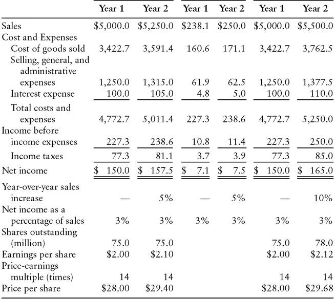
In the fictitious example in Exhibit 3.5, Big Time Corp.’s sales increase by 5% between Year 1 and Year 2. Small Change, a smaller, privately owned company in the same industry, also achieves 5% year-over-year sales growth. Suppose now that at the end of Year 1, Big Time acquires Small Change with shares of its own stock. The Big Time income statements under this assumption (“Acquisition Scenario”) show a 10% sales increase between Year 1 and Year 2. (Note that Year 1 is shown as originally reported, with Small Change still an independent company, while in Year 2, the results of the acquired company, Small Change, are consolidated into the parent’s financial reporting. Analysts might also examine a pro forma income statement showing the levels of sales, expenses, and earnings that Big Time would have achieved in Year 1, if the acquisition had occurred at the beginning of that year.)
On the face of it, a company growing at 10% a year is sexier than one growing at only 5% a year. Observe, however, that Big Time’s profitability, measured by net income as a percentage of sales, does not improve as a result of the acquisition. Combining two companies with equivalent profit margins of 3% produces a larger company that also earns 3% on sales. Shareholders do not gain anything in the process, as the supplementary figures in Exhibit 3.5 demonstrate.
If Big Time decides not to acquire Small Change, its number of shares outstanding remains at 75.0 million. The earnings increase from $150.0 million in Year 1 to $157.5 million in Year 2 raises earnings-per-share from
EXHIBIT 3.5 Sales Growth Acceleration without Profitability Improvement Big Time Corporation and Small Change, Inc.—Illustration ($000 omitted)
Nonacquisition Acquisition
Scenario Scenario
Big Time Small Big Time
Corporation Change Inc. Corporation
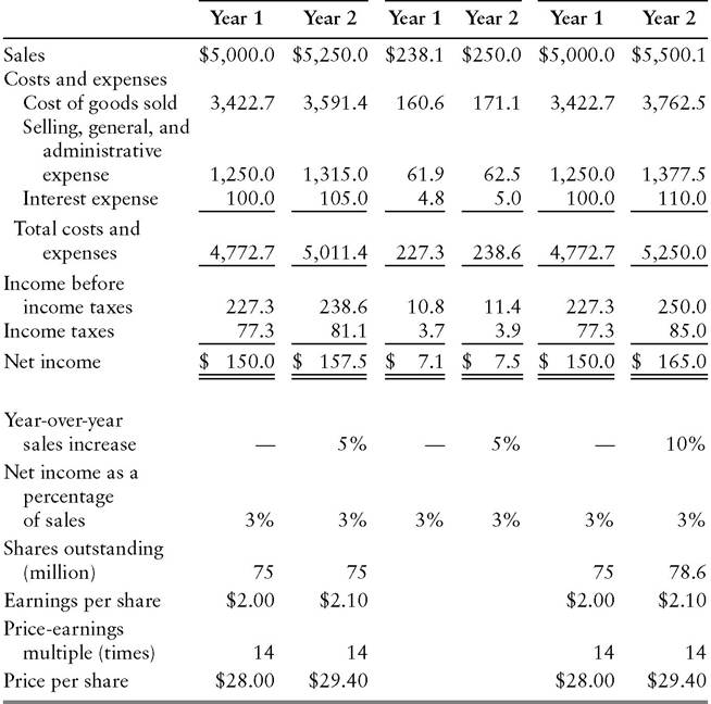
$2.00 to $2.10. With the price-earnings multiple constant at 14 times, equivalent to the average of the company’s industry peers, Big Time’s stock price rises from $28.00 to $29.40 a share.
In the Acquisition Scenario, on the other hand, Big Time pays its industry-average earnings multiple of 14 times for Small Change, for a total acquisition price of $7.1 million × 14 = $99.4 million. At Big Time’s Year 1 share price of $28.00, the purchase therefore requires the issuance of $99.4 million ÷ $28.00 = 3.6 million shares. With the addition of Small Change’s net income, Big Time earns $165.0 million in Year 2. Dividing that figure by the increased number of shares outstanding (78.6 million) produces earnings per share of $2.10. At a price-earnings multiple of 14 times, Big Time is worth $29.40 a share, precisely the price calculated in the Nonacquisition Scenario. The mere increase in annual sales growth from 5% to 10% has not benefited shareholders, whose shares increase in value by 5% whether Big Time acquires Small Change or not.
Analysts should note that this analysis is sensitive to the assumptions underlying the scenarios. Suppose, for instance, that Big Time finances the acquisition of Small Change with borrowed money, instead of issuing stock. Let us suppose that Big Time must pay interest at a rate of 8% on the $99.4 million of new borrowings. Interest expense in Year 2 of the Acquisition Scenario is now $118.0 million, rather than $100.0 million. Pretax income therefore falls from $250.0 million to $242.0 million, reducing net income from $165.0 million to $159.7 million at the company’s effective tax rate of 34%. Only 75.0 million shares are outstanding at the conclusion of the transaction, however, rather than the 78.6 million observed in the acquisition- for-stock case. As a result, Big Time’s earnings per share rise to $159.7 million ÷ 75.0 million = $2.13.
style='text-indent:18.0pt'>Assuming the market continues to assign a multiple of 14 times to Big Time’s earnings, the stock is now worth $29.82, a bit more than in the Nonacquisition Scenario. In practice, the investors may reduce Big Time’s price-earnings multiple slightly to reflect the heightened risk represented by its decreased interest coverage. (Following the formulas laid out in Chapter 13, income before interest and taxes declines from $360.0 million ÷ $110.0 million = 3.3 times in the stock-acquisition case to $360.0 million ÷ $118.0 million = 3.1 times in the debt-financed-acquisition case.) If the priceearnings multiple falls only from 14 to 13.8 times as a result of this decline in debt protection, Big Time’s stock price in this variant again comes to $29.40, equivalent to the Year 2 price in the Nonacquisition Scenario. As in the case of Big Time paying with stock for the acquisition of Small Change, shareholders do not benefit if Big Time instead borrows the requisite funds, assuming investors are sensitive to the impact of the company’s increased debt load on its credit quality.Internal versus External Growth
More important than the fine-tuning of the calculations is the principle that a company cannot truly increase shareholders’ wealth by accelerating its revenue growth without also improving profitability. This does not dissuade companies from attempting to mesmerize analysts with high rates of sales growth generated by grafting other companies’ sales onto their own through acquisitions. Analysts may fall for the trick by failing to distinguish between internal growth and external growth.
Internal growth consists of sales increases generated from a company’s existing operations, while the latter represents incremental sales brought in through acquisitions. An internal growth rate greater than the average recorded for the industry implies that the company is gaining market share from its competitors. As a precaution, the analyst must probe further to determine whether management has merely increased unit sales by accepting lower gross margins. If that is not the case, however, the company may in fact be improving its competitive position and, ultimately, increasing its value. On the other hand, if Company A generates external growth by acquiring Company B and neither Company A nor its new subsidiary increases its profitability, then the intrinsic value of the merged companies is no greater than the sum of the two companies’ values.
External growth can increase shareholders’ wealth, however, if the mergers and acquisitions lead to improvements in profitability. This effect is commonly referred to as synergy. It is a term much abused by companies that promise to achieve operating efficiencies, without offering many specific examples, through acquisitions that appear to offer few such opportunities. Nevertheless, even analysts who have grown cynical after years of seeing purported synergies remain unrealized will acknowledge the existence of several bona fide means of raising a company’s profit margins through external growth.
For one thing, a company may be able to reduce its cost per unit by increasing the size of its purchases. Suppliers commonly offer volume discounts to their large customers, which they can service more efficiently than customers who order in small quantities. If the cost of materials, fuel, and transportation required to produce each widget goes down while the selling price of widgets remains unchanged in a stable competitive environment, the company’s gross margin increases.
Another way to increase profitability through external growth involves economies of scope. In a simple illustration, a manufacturer of potato chips has a sales force calling on retail stores. Much of the associated expense represents the time and transportation costs incurred as the salespeople travel from store to store, as well as the salespeople’s health insurance and other benefits. Now suppose that the potato chip manufacturer acquires a pretzel manufacturer. For the sake of explication, assume that the pretzel company formerly relied on food brokers, rather than an in-house sales force. The acquiring company terminates the contracts with the brokers and adds pretzels to its potato chip sales force’s product line. Revenues and gross profits per sales call rise with the addition of the pretzel line. The number of sales calls per salesperson remains essentially constant, because taking orders for the additional product consumes little time. Accordingly, time and transportation costs per sales call do not rise materially, while the cost of health insurance and other benefits does not rise at all. Adding it all up, the profitability of selling both potato chips and pretzels through the same distribution channel is greater than the profitability of selling one snack food only.
Analysts should be forewarned that claims of potential economies of scope often prove, in retrospect, to be exaggerated. Over a period of several decades, for example, banks, brokerage houses, and insurance companies have frequently proclaimed the advent of the “financial supermarket,” in which a single distribution channel will efficiently deliver all classes of financial services to consumers. A fair amount of integration between these businesses has certainly occurred, but cultural barriers between the businesses have turned out to be more formidable than corporate planners have foreseen. Considerable training is required to teach salespeople how to shift gears between the fast-paced business of dealing in stocks and the more painstaking process of selling insurance policies. In general, the less closely related the combining businesses are, the less certain it is that the hoped-for economies of scope will be realized. When disparate companies combine in pursuit of novel synergies, analysts should treat with extreme caution the margin increases shown in pro forma income statements produced by management.
Capturing Economies of Scale
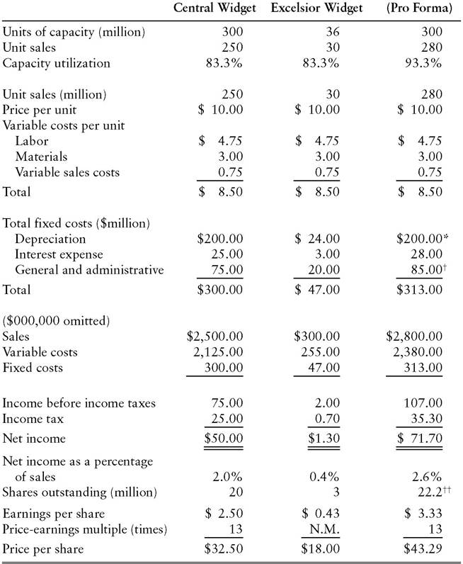
color=black face="Times New Roman">Finally, and perhaps most famously, mergers can genuinely increase profitability and shareholder wealth through economies of scale. As illustrated in Exhibit 3.6, Central Widget is currently utilizing only 83.3% of its productive capacity. At the present production level, the company’s fixed costs amount to $300 million ÷ 250 million = $1.20 per unit, or 12% of each sales dollar. These irreducible costs represent a major constraint on the company’s net profit margin, just 2.0%, and in turn its return on equity (see Chapter 13), which is an unexciting 11.1%.
Central Widget spies an opportunity in the form of its smaller competitor, Excelsior Widget. Because the two companies operate in the same geographic region, it would be feasible to consolidate production in Central Widget’s underutilized factories. Management proposes a merger premised on achieving economies of scale.
Excelsior’s cost structure is similar to Central’s, except that its general and administrative expense is higher as percentage of sales (6.7% versus
EXHIBIT 3.6 Economies of Scale (Illustration)
Selected Production and Financial Statement Data
Central Widget
*Assumes closure of Excelsior Widget factory.
+Assumes elimination of 50% of Excelsior Widget’s general and administrative expense through closure of company headquarters.
++Assumes acquisition price of $23.40 per Excelsior Widget share.
3.0%). The problem is that certain costs (such as the upkeep on a headquarters building and salaries of senior executives) are nearly as great for Excelsior as for Central, but Excelsior has a smaller base of sales over which to spread them. As a result, Excelsior is running at a loss at current operating levels. Its board of directors therefore accepts the acquisition offer. Central pays $23.40 worth of its own stock (0.72 shares) for each share of Excelsior, a 30% premium to Excelsior’s prevailing market price.
Unlike the acquisition of Small Change by Big Time depicted in Exhibit 3.5, this transaction not only increases the acquiring company’s sales, but also improves its profitability. Following the acquisition, on a pro forma basis, Central Widget’s fixed cost per unit is $313.0 million ÷ 280 million = $1.12, down from $1.20. The net margin is up from 2.0% to 2.6%, while earnings per share have jumped from $2.50 to $3.33, pro forma. If the market continues to assign a multiple of 13 times to Central’s earnings, the stock should theoretically trade at $43.29, up from $32.50 before the transaction. Realistically, that increase probably overstates the actual rise that Central Widget shareholders can expect. Aside from severance costs not shown in the pro forma income statement, investors may reduce the priceearnings multiple to reflect the myriad uncertainties faced in any merger, such as potential loss of key p ersonnel and the predictable traumas of melding distinct corporate cultures. After all the dust has settled, however, Central Widget’s shareholders will assuredly benefit from the economies of scale achieved through the acquisition of Excelsior Widget.
Scale economies become available for a variety of reasons. Technological advances can make a sizable portion of existing capacity redundant. For example, computerization has increased the productivity of financial services workers engaged in clearing transactions. Consolidation in the banking and brokerage industries has been hastened by cost savings achievable through handling two companies’ combined volume of transactions with fewer back office workers than the companies previously employed in aggregate.
Economies of scale also arise through consolidation of a “mom-and- pop” business, that is, an industry characterized by many small companies operating within small market areas. For example, waste hauling has evolved from a highly localized business to an industry with companies operating on a national scale. Among the associated efficiencies is the ability to reduce garbage trucks’ idle time by employing them in several adjacent municipalities.
Behind the Numbers: Fixed versus Variable Costs
As synergies go, projections of economies of scale in combinations of companies within the same business tend to be more plausible than economies of scope purportedly available to companies in tangentially connected businesses. The existence of chronically underutilized capacity is apparent to operations analysts within corporations and to outside management consultants. Word inevitably spreads from there until the possibility of achieving sizable efficiencies through consolidation becomes common knowledge among investors. Companies’ published financial statements typically provide too little detail to quantify directly the potential for realizing economies of scale.
Companies do not generally break out their fixed and variable costs in the manner shown in Exhibit 3.6. Instead, they include a combination of variable and fixed costs in cost of goods sold. Somewhat helpfully, the essentially fixed costs of depreciation and interest app ear as separate lines. On the whole, however, a company’s published income statement provides only limited insight into its operating leverage, or the rate at which net income escalates once sales volume rises above the breakeven rate. This is unfortunate, because a breakout of fixed and variable costs would be immensely helpful in quantifying the economies of scale potentially achievable through a merger. More generally, such information would greatly facilitate the task of forecasting a company’s earnings as a function of projected sales volume.
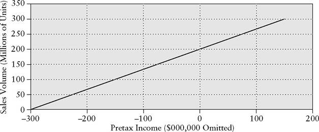
Exhibit 3.7 uses data from the Central Widget example to plot the relationship between sales volume and pretax income (income before income taxes). The company breaks even at a sales volume of 200 million units, the level at which the $1.50 per unit contribution (margin of revenue over variable cost) exactly offsets the $300 million of fixed costs. Once fixed costs are covered, the contribution on each incremental unit sold flows directly to the pretax income line. At full capacity, 300 million units, Central Widget earns $150 million before taxes. (Note that analysts can alternatively remove interest expense from the calculation and base a breakeven analysis on operating income.)
In theory, an analyst can back out the fixed and variable components of a company’s costs from reported sales and income data. The object is to produce a graph along the lines of the one shown in Exhibit 3.7, while also estimating the contribution per unit. At that point, the analyst can create a table like that shown in the exhibit and establish the sensitivity of profits to the portion of capacity being utilized.
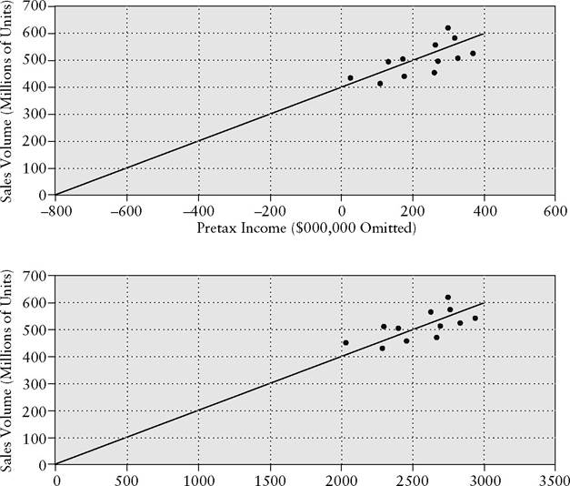
Exhibit 3.8 presents the fictitious case of West Coast Whatsit. The top graph plots the company’s reported unit sales volume versus pretax income for each of the past 10 years. (West Coast is debt-free and has no other nonoperating income or expenses, so the company’s operating income is equivalent to its pretax income.) Observe that the plotted points are concentrated in the upper right-hand corner of the graph, reflecting that annual sales
EXHIBIT 3.7 Operating Leverage—Illustration Central Widget
|
| Contribution |
| Fixed | Pretax |
| Units * | per Unit = | Contribution | — Costs | = Income |
| 300 | $1.50 | $450 | size=1 color=black face="Times New Roman">$300 | $150 |
| 250 | 1.50 | 375 | 300 | 75 |
| 200 | 1.50 | 300 | 300 | 0 |
| 150 | 1.50 | 225 | 300 | (75) |
| 100 | 1.50 | 150 | 300 | (150) |
| 50 | 1.50 | 75 | 300 | (225) |
| 0 | 1.50 | 0 | 300 | (300) |
(Units in millions. Contribution, fixed costs, and pretax income in millions of dollars.)
size=3 color=black face="Microsoft Sans Serif">
![]()
volume never declined to less than 380 million units (63% of capacity) during the period. At that low ebb, pretax income fell below zero.
The next step is to fit a diagonal line through the points, as shown in the upper graph. (For a precise technique of fitting a line, see the discussion of the least-squares method in Chapter 14.) According to the line derived from the empirical observations, the company’s breakeven sales volume is 400 million units, that is, the point on the diagonal line that corresponds to zero on the horizontal scale (pretax income). Although West Coast Whatsit has not utilized 100% of its capacity in any of the past 10 years, the graph indicates that at that level (600 million on the vertical scale), pretax income would amount to $400 million.
To complete the analysis, the analyst must also plot the reported unit sales volume versus dollar sales for the past 10 years, as shown in the lower graph. The remaining task is to back into the data required to fill in the
EXHIBIT 3.8 Backing out Fixed and Variable Costs—Illustration West Coast Whatsit
Sales ($000,000 Omitted)
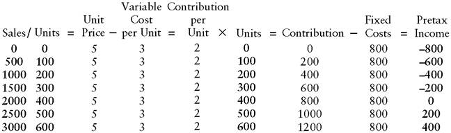
table at the bottom of Exhibit 3.8. At the outset, the analyst knows only the figures shown in boldface, which can be derived directly from the two graphs. For example, the fitted line shows that at full capacity (600 million units), sales would total $3.0 billion.
According to the known data, the increase in pretax income between the breakeven volume (400 million units) and a volume of 500 million units is $200 million. That dollar figure must represent the contribution on 100 million units. Dividing $200 million by 100 million yields the contribution per unit of $2.00, enabling the analyst to fill in that whole column. Dividing any figure in the sales column by its corresponding number of units (e.g., $2.5 billion and 500 million) provides the unit price of $5.00, which goes on every line in that column. Cost per unit, by subtraction, is $3.00.
At the breakeven level (pretax income = $0), contribution totals 400 million units times $2.00 = $800 million. The analyst can put that number on every line in the entire Fixed Costs column. All that remains is to fill in the Contribution column by multiplying each remaining line’s number of units by the $2.00 contribution per unit figure.
Regrettably, the elegant procedure just described tends to be highly hypothetical, even though it is useful to go through the thought process. To begin with, companies engaged in a wide range of products do not disclose the explicit unit volume figures that the analysis requires. Relating their sales volumes to prices and costs is more complicated than in the case of a producer of a basic metal or a single type of paper. The Management Discussion and Analysis section of a multiproduct company’s financial report may disclose period-to-period changes in unit volume, but not absolute figures, by way of explaining fluctuations in revenues. A rise or drop in revenue, however, may also reflect changes in the sales price per unit, which may in turn be sensitive to industrywide variance in capacity utilization. In addition, revenue may vary with product mix. When a recession causes consumers to turn cautious about spending on major appliances, for example, they may trade down to lower-priced models that provide smaller contributions to the manufacturers. Finally, multiproduct companies’ product lines typically change significantly over periods as long as the 10 years assumed in Exhibit 3.8.
For all these reasons, analysts generally cannot back out fixed and variable costs in practice. When projecting a company’s income statement for the coming year, they instead work their way down to the operating income line by making assumptions about cost of goods sold (COGS) and selling, general, and administrative expenses (SG&A) as percentages of sales (see Chapter 12). They try in some sense to take into account the impact of fixed and variable costs, but they cannot be certain that their forecasts are internally consistent.
In Exhibit 3.8, total pretax costs are equivalent to the sum of COGS and SG&A. (Remember that West Coast Whatsit has no interest expense or other nonoperating items.) An analyst who projects that the two together will represent 92% of sales is making a forecast consistent with sales volume of 500 million units, or 83% of capacity. At that unit volume, variable costs total 500 million × $3.00 = $1.5 billion, which when added to fixed costs of $800 million, produces total costs of $2.3 billion, or 92% of sales measuring $2.5 billion. The assumption of a total pretax cost 92% ratio would be too pessimistic if the analyst actually expected West Coast to operate in line with the whatsit industry as a whole at 90% of capacity. That would imply unit sales of 540 million, resulting in variable costs of $1.62 billion and total costs of $2.42 billion. The ratio of operating expenses to sales of $2.7 billion (540 million units @ $5.00) would be only 90%. Observe that not only operating income, but also the operating margin rises as sales volume increases.
Estimating COGS and SG&A as percentages of sales is an imperfect, albeit necessary, substitute for an analysis of fixed and variable costs. Conscientious analysts must strive to mitigate the distortions introduced by the shortcut method. They should avoid the trap of uncritically adopting the projected COGS and SG&A percentages kindly provided by companies’ investor relations departments. Analysts who do so risk sacrificing their independent judgment. After all, the preceding paragraph demonstrates that a forecast of the operating margin must reflect an implicit assumption about sales volume. Accordingly, a company’s “guidance” regarding COGS and SG&A percentages necessarily incorporates management’s assumption about the coming year’s sales volume. At the risk of stating the obvious, management’s embedded sales projection will often be more optimistic than the analyst’s independently generated forecast.
Readers should not infer from the absence of disclosure about fixed and variable costs that the information is unimportant to understanding companies’ financial performance. On the contrary, a company’s fixed-variable mix can be a dominant factor in analyzing both its credit quality and its equity value (see Chapters 13 and 14, respectively). A company with relatively large fixed costs has a high breakeven level. Even a modest economic downturn will reduce its capacity utilization below the rate required to keep the company profitable. A cost structure of this sort poses a substantial risk of earnings falling below the level needed to cover the company’s interest expense. On the other hand, if the same company has low variable costs, its earnings will rise dramatically following a recession. Each incremental unit of sales will contribute prodigiously to operating income. Two real-life examples demonstrate the analytical value of understanding the fixed-versus- variable nature of a company’s cost structure, even though it may not be feasible to document the mix precisely from the financial statements.
As an amusement park operator, Six Flags exemplifies the high-fixed- cost company. Attendance (and therefore revenue), shows wide seasonal variations, but the company’s costs are concentrated in categories that do not vary with attendance. Examples include occupancy, depreciation on rides, insurance, and wages of employees who must be on site whether the parks are full or nearly empty.
A time series of the company’s cost of sales as a percentage of sales (Exhibit 3.9) shows wide quarterly fluctuations, largely reflecting extreme seasonality in the company’s business. In 2000, for example, the warmweather second and third calendar quarters accounted for more than 90% of the parks’ attendance. During those two quarters, which perennially contribute the vast majority of annual revenues, cost of sales runs less than 50% of revenues. In the cold-weather quarters ending December 31 and March 31, by contrast, the ratio soars to over 100%. Year-over-year variances in profit margins, also arising from wide fluctuations in attendance, are substantial as well. Cost of sales soared to 272% of sales in the quarter ending December 31, 1996, but measured only 109% in the corresponding quarter of 1999.
Washington Group International, known as Morrison Knudsen during most of the period shown in Exhibit 3.10, represents the opposite extreme in
EXHIBIT 3.9 Six Flags, Inc. Cost of Sales as a Percentage of Sales. Quarterly 1996-2000.
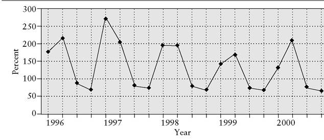
Source: Compustat.
EXHIBIT 3.10 Washington Group International, Inc. Cost of Sales as a Percentage of Sales. Quarterly 1996-2000.
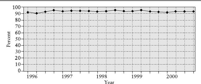
Source: Compustat.
cost structures. The engineering and construction concern incurs variable labor and material costs with each contract it obtains. Once Washington Group completes the project, the associated costs cease. If the volume of available work declines from one year to the next, the company’s total costs decline nearly in proportion, as fixed costs are too low to have a large impact.
Consistent with this qualitative description of Washington Group’s mix of fixed and variable costs, the company’s cost of sales as a percentage of sales scarcely budges from period to period. The ratio consistently ran between 90% and 95% from 1996 through 2000. In the quarter ending December 31, 1997, the percentage was identical to the preceding quarter’s, at 94.0%. Similar quarter-to-quarter stability, at the 93.9% level, was observed in the successive quarters ending December 31, 1998 and March 31, 1999.
Credit analysts ordinarily perceive substantial risk in the sort of high- fixed-cost pattern revealed by the Six Flags graph in Exhibit 3.9. Even a comparatively modest drop in revenue and, by extension, contribution can drive operating income below the level required to cover interest expense. By contrast, a highly variable cost structure like Washington Group’s inherently provides a great deal of financial flexibility. With few other fixed costs to meet in the event of a revenue decline, an engineering and construction company ought to be able to stay current on its interest expense, provided it keeps its debt burden at a prudent level.
Surprisingly, however, Washington Group defaulted on its debt and filed for bankruptcy in May 2001. The action followed a severe liquidity squeeze arising from unprofitable contracts that the company took over in connection with its April 2000 acquisition of Raytheon Engineers & Constructors (RE&C). In response to the credit crisis, Washington Group halted certain work on two major projects related to the acquisition and sued the seller of RE&C, Raytheon Company, alleging fraud and breach of contract.
Washington Group’s sudden descent into bankruptcy did not negate the general rule that a predominantly variable cost structure aids financial flexibility. Rather, the lesson for students of financial statements was the possibility of discontinuities in any company’s earnings record. Ordinarily, the sort of consistency in profit margins depicted in Exhibit 3.10 is reassuring to credit analysts, but they must never feel reassured to the point of complacency.
Playing with Price-Earnings Multiples
Vigilance, as exemplified by the need to watch for earnings discontinuities, has been a recurring theme throughout this exploration of the ins and outs of income statements. Other pitfalls to watch out for include unrealizable synergies and company-furnished projections of cost ratios that incorporate management’s assumptions regarding sales volume. Before moving on, vigilant analysts should familiarize themselves with a device that companies have developed to get around the general proposition that mergers do not increase value unless they increase profitability.
Turning back to the fictitious acquisition case presented in Exhibit 3.5, let us change one assumption (see Exhibit 3.11). As a comparatively small company within its industry, Small Change probably will not command as high a price-earnings multiple as its larger industry peers. Therefore, we shall assume that Big Time is able to acquire the company for only 12 times earnings, rather than 14 times, as indicated in Exhibit 3.5.
Our revised assumption does not alter the income statements in either year under either the Acquisition or Nonacquisition Scenario. The acquisition price, however, falls from $99.4 million to $7.1 million x 12 = $85.2 million. Big Time issues only $85.2 million ÷ $28.00 = 3.0 million shares to pay for the acquisition, rather than 3.6 million under the previous assumption. Consequently, Big Time has 78.0 million shares outstanding at the end of Year 2 under the Acquisition Scenario, instead of 78.6 million. Earnings per share come to $165.0 million ÷ 78.0 million = $2.12. At a price-earnings multiple of 14 times, Big Time’s stock is valued at $29.68 a share following the Small Change acquisition, slightly higher than the $29.40 figure shown in the Nonacquisition Scenario. Big Time could vault its share price to a considerably loftier level by making a series of acquisitions on a similar basis.
In contrast to the outcome depicted in Exhibit 3.5, Big Time increases the value of its stock through the acquisition of Small Change. The company
EXHIBIT 3.11 Exploiting a Difference in Price-Earnings Multiples Big Time Corporation and Small Change, Inc.—Illustration ($000 omitted)
Nonacquisition Acquisition
Scenario Scenario
Big Time Small Big Time
Corporation Change, Inc. Corporation
achieves this effect without realizing operating efficiencies through the combination. Following the transaction, Big Time’s ratio of net income to sales is 3%, unchanged from its preacquisition level.
The rational explanation of this apparent alchemy lies in Big Time’s ability to exchange its stock for shares of privately owned Small Change on highly favorable terms. By acquiring the smaller company at a price of 12 times earnings with stock valued at a multiple of 14 times, Big Time spreads Small Change’s earnings across fewer shares than would be the case if the market valued the two companies at the same multiple. The effect, achieved purely through financial engineering, is a parody of the economies of scale realized in mergers premised instead of improvements in operations.
In fairness to the many real-world companies that have exploited disparities in price-earnings multiples over the years, Big Time’s share-priceenhancing acquisition rests squarely within the bounds of fair play. Companies legitimately take advantage of favorable currency exchange rates when deciding whether to purchase materials and equipment domestically or overseas. If the dollar is high relative to the Euro, companies based in the United States can source goods more economically in Europe than at home. In principle, it is no less appropriate or beneficial to shareholders to buy earnings with a highly valued “acquisition currency,” that is, its own stock.
Furthermore, as shareholders of a private company, Small Change’s owners do not have to be coerced to sell out to Big Time. The disparity in price-earnings multiples is justified by the private company’s owners’ opportunity to exchange an illiquid investment for public stock, for which a deep and active trading market exists. If anything, the difference between Big Time’s multiple of 14 times and Small Change’s 12 times understates the valuation gap between the public and private shares. Lacking a secondary market that would reward higher reported income with a higher share price, private owner-managers commonly extract compensation through perquisites that their companies can lawfully account for as business expenses. The result is lower net income than comparably successful public companies would report, but with the value of the “perks” delivered on a pretax basis. Instead of buying cars with dividends distributed from aftertax income, the owner-managers can drive fancier, more expensive company- provided cars purchased with pretax dollars. After adjusting Small Change’s reported income for expenses that would not be incurred at a public company such as Big Time, the $85.2 million acquisition price might represent a multiple of only 10 or 11 times, rather than 12 times.
In short, there is nothing inherently unsavory about paying for low- multiple companies with high-multiple stock. Why, then, does the technique warrant special focus in a chapter covering the broad subject of income statements? The answer is that like many other legitimate financial practices, exploiting disparities in price-earnings multiples is prone to abuse. Capitalizing on disparities in price-earnings multiples can lead to trouble in several ways.
To begin with, suppose a high-multiple company acquires a low- multiple company during a period of exceptionally wide dispersion in valuations. In a shift from normal conditions to a “two-tiered” market, the respective multiples might go, for sake of example, from 15 and 12 to 25 and 10. Selling stockholders of the low-multiple company would likely consider it a fair exchange to accept payment in shares of the high-multiple company at the prevailing market price. Their feelings would probably change dramatically, however, if the two-tiered market abruptly ended with the purchaser’s stock receding from 25 times earnings to a more ordinary 15 times. Sellers who retained the acquiring company’s shares would discover that their value received had suddenly fallen by 40%. (It is reasonable to assume that many shareholders would have held on to the shares, because doing so would ordinarily delay the incurrence of capital gains taxes on the sale. Unlike cash-for-stock transactions, stock-for-stock acquisitions generally qualify as tax-free exchanges.)
Readers might accuse the selling shareholders of being crybabies. After all, they knew when they accepted the acquiring company’s shares as payment that they would be exposed to stock market fluctuations, much as they were prior to the deal. The difference, however, is that if they had held onto their low-multiple stock, their loss would not have been 40%, but only 17%, that is, from 12 times to 10 times earnings. (A complete comparison must also take into account any premium over the previously prevailing stock price received by the selling shareholders.)
Financial statement analysis would not have warned the selling shareholders of the impending marketwide drop in price-earnings multiples. Careful scrutiny of the acquiring company’s income statement might very well have determined, however, that its shares were susceptible to a sharp decline. Over the years, many voracious acquirers have temporarily achieved stratospheric multiples on their acquisition currency through financial reporting gimmicks that hard-nosed analysts were able to detect before the share prices fell back to earth.
In some instances, the basis for an exaggerated P/E multiple is rapid earnings per share growth achieved through financial engineering, rather than bona fide synergies. Starting with a modest multiple on its stock, a company can make a few small acquisitions of low-multiple companies to get the earnings acceleration started. Each transaction may be too small to be deemed material in itself. That would eliminate any obligation on the company’s part to divulge details that would make it easy for analysts to quantify the impact of the company’s exploitation of disparities in P/E multiples. As quarter-to-quarter percentage increases in EPS escalate, the company’s equity begins to be perceived as a high-growth glamour stock. Obliging investors award the stock a higher multiple, which increases the company’s ability to buy earnings on favorable terms. Management may succeed in pumping up the P/E multiple even further by asserting that it can achieve economies of scope through acquiring enterprises outside, yet in some previously unrecognized way, complementary to the company’s core business.
The conglomerate craze of the 1960s relied heavily on these techniques, and with variations, they have been reused in more recent times. Massive declines in the share prices of the insatiable acquirers’ stock prices have frequently resulted. Contributing to the downslides have been the practical problems of integrating the operations of diverse companies. Deals that work on paper have often foundered on incompatible information systems, disparate distribution channels, clashes of personality among senior executives, and contrasting corporate cultures. In addition, the process of boosting earnings per share through acquisition of lower-multiple companies may prove unsustainable. For example, if competition heats up among corporations seeking to grow through acquisition, the P/E gap between acquirers and target companies may narrow. That could get in the way of the continuous stream of acquisitions needed to maintain EPS growth in the absence of profit improvements. Inevitably, too, the voracious acquirer will suffer a normal cyclical decline in the earnings of its existing operations. The company’s price-earnings multiple may then decline relative to the multiples of its potential targets, interrupting the necessary flow of acquisitions.
It is no small task to dissect the income statement of a corporation that makes frequent acquisitions and discloses as few details as possible. Nevertheless, an energetic analyst can go a long way toward segregating ongoing operations from purchased earnings growth. Acquisitions of public companies leave an information trail in the form of regulatory filings. Conscientious searching of the media, including the industry-specialized periodicals and local newspapers, may yield useful tidbits on acquisitions of private companies. Such investigations will frequently turn up the phrase, “terms of the acquisition were not disclosed,” but reliable sources may provide informed speculation about the prices paid. Finally, the acquirers may furnish general information regarding the range of earnings multiples paid in recent deals. If an analysis of the available data indicates that management is expanding its empire without creating additional value through genuine economies of scale or scope, the prudent action is to sell before the bottom falls out.
Is Fraud Detectable?
As a final point on the reality underlying the numbers, readers should note that although the tactics detailed in the preceding discussion may not win awards for candor in financial reporting, neither will most of them land corporate managers in the p enitentiary. Analysts must be mindful that there are many ways for companies to pull the wool over investors’ eyes without fear of legal retribution. Sometimes, however, corporate executives step over the line into illegality.
Outright misrepresentation falls into a category entirely separate from the mere exploitation of financial reporting loopholes. Moreover, the gravity of such misconduct is not solely a matter of temporal law. In 1992, the Roman Catholic Church officially classified fraudulent accounting as a sin. A catechism unveiled in that year listed book-cooking in a series of “new” transgressions, that is, offenses not known in 1566, the time of the last previous overhaul of church teachings.
Neither fear of prosecution nor concern for spiritual well-being, however, entirely deters dishonest presenters of financial information. Audits, even when conducted in good faith, sometimes fail to uncover dangerous fictions. Financial analysts must therefore strive to protect themselves from the consequences of fraud.
No method is guaranteed to uncover malfeasance in financial reporting, but neither are analysts obliged to accept a clean auditor’s opinion as final. Even without the resources that are available to a major accounting firm, it is feasible to find valuable clues about the integrity of financial statements.
Messod Daniel Beneish, Professor of Accounting and Information Systems at the Kelley School of Business at Indiana University, has developed a model for identifying companies that are likely to manipulate their earnings, based on numbers reported in their financial statements.17 (Beneish defines manipulation to include both actual fraud and the management of earnings or disclosure within GAAP. In either case, his definition specifies that the company subsequently must have been required to restate results; write off assets; or change its accounting estimates or policies at the behest of its auditors, an internal investigation, or a Securities and Exchange Commission probe.) Beneish finds, by statistical analysis, that the presence of any of the following five factors increases the probability of earnings manipulation:
1. Increasing days sales in receivables.
2. Deteriorating gross margins.
3. Decreasing rates of depreciation.
4. Decreasing asset quality (defined as the ratio of noncurrent assets other than property, plant, and equipment to total assets).
5. Growing sales.
Note that Beneish does not characterize these indicators as irrefutable evidence of accounting malfeasance. Indeed, it would be disheartening if every company registering high sales growth were shown to be achieving its results artificially. Nevertheless, Beneish’s data suggest a strong association between the phenomena he lists and earnings manipulation.
More on the topic HOW REAL ARE THE NUMBERS?:
- Conclusion
- Indirect but Theory-Free Observation
- Legal Aid and the Bar, from Symbiosis to Parasitism
- THE THEORY AND PRACTICE OF EMPIRE-BUILDING
- The Netherlands and the UK: The Witteveen Reports and their contradictory results
- Article 6.8 Great Portland strikes with convertible bond
- From the 1940s to 1960s, Pakistan moved from being under British colonial rule to coming under the influence of the United States (U.S.).
- Testate Succession
- REVIEW OF FORENSIC ASSESSMENT INSTRUMENTS
- Legal battlefields after the 1994 genocide In Rwanda