Adaptive movements and their effects on competition
10.5.1 General aspects of adaptive movement
The first treatment of adaptive movement was by Steven Fretwell (1972; also Fretwell and Lucas 1969), who introduced the term ‘ideal free distribution’ to describe the endpoint of this process.
This was a distribution of individuals across patches that was characterized by equal fitness (instantaneous per capita growth rate) in all occupied patches, with occupied patches characterized by greater fitness than a single individual would achieve in an unoccupied patch. ‘Ideal’ referred to complete and accurate information about conditions, while ‘free’ referred to the lack of any cost to movement. Both of these defining characteristics are difficult to achieve precisely in real systems, but spatial distributions close to ideal free have often been observed in various behavioural studies (reviewed in Milinski and Parker 1991; Giraldeau and Caraco 2000). If such ‘ideal free distributions’ (IFDs) are common, it could be because movement at fixed condition-independent rates is a special case that seldom occurs in natural systems. However, there is still considerable debate about the prevalence of IFDs (Matsumura et al. 2010). Lack of IFDs could be due to movement that is not sufficiently rapid, species that are poor at detecting resource abundances, or rapidly fluctuating conditions. General evolutionary considerations suggest that both consumers and living resources should behave adaptively, and it is not obvious whether their combined movements will come to some equilibrium. This implies the need for dynamic models of movement. Fretwell (1972) did not discuss the details ofindividu- al movement decisions that would be needed to approximate an ideal free distribution in such a case. Some of the subsequent work on this issue is discussed later in this section. Much work on IFDs has assumed that only a single consumer species was present, but this is unlikely for most species in natural communities.The mechanistic basis of adaptive movement has received some attention in recent years, but empirical results are scarce, and there is little agreement on a quantitative description of the process. The simplest case is again one with two patches. This scenario has many similarities to adaptive choice between two types of behaviours in a homogeneous system. It is known that adaptive consumer diet choice in a homogeneous (single patch) system often alters intraspecific and interspecific competition (Abrams and Matsuda 2004; Abrams 2006a, b). Adaptive diet choice within a habitat has often been assumed to occur instantaneously with changes in prey or resource abundances; this is true of early models of ‘switching’ behaviour (Murdoch and Oaten 1975). However, this assumption is biologically unlikely, and it can produce very different dynamics than models with explicit behavioural dynamics (Abrams 1999, 2000b, 2007a; Abrams and Matsuda 2003,2004). Similarly, understanding movement between patches also requires consideration of the dynamics of the movement process. Adaptive movement by the resources, when they are biological entities, usually depends on the abundances of their own resources, as well as the risk of being eaten by consumers. Understanding spatially structured interactions between the consumers of such living resources is therefore likely to require a model representing three trophic levels explicitly, and having movement rates that can potentially depend on the abundances of all three levels.
Species are likely to exhibit a net movement toward patches with better conditions than their current patch, but it is unclear how often they have information that would enable them to accurately estimate their future demographic parameters in other places. Resource abundance is one of the primary quantities likely to affect movement. Sufficiently low resource abundance for a consumer in its current patch is likely to imply that conditions might be better elsewhere, so adaptive movement could be based solely on the current or recent conditions in the occupied patch.
However, long-distance detection of resource abundances in other patches is likely to be possible in some cases, and, as noted above, short visits to a nearby patch maybe rapid enough for a model to ignore, provided the species returns to its original patch after a visit to a patch with poorer conditions. Thus, the instantaneous fitness associated with original and potential destination patches should both frequently affect the movement rate.The models explored below assume that consumers and/or resources move at a rate that is an accelerating function of the fitness difference implied by moving between patches. The accelerating nature of the relationship is based on the fact that both the ability to detect differences, and the reward from moving increase with the fitness difference. Larger fitness differences also imply that the relative ranking of the two patches is likely to persist for a longer time. The specific function used in the numerical analysis here is that proposed in Abrams (2000b): the consumer per capita movement rate from patch i to patch j, Mij, is given by,
Mij = mExp[λ(Wj — Wi)], (10.5)
where the parameter m gives the between-patch movement rate when patches yield equal fitness change per unit time (and hence, random movement). The parameter λ is a positive constant that scales movement propensity to the difference in fitness, measured by instantaneous per capita growth rate, W. Equation (10.5) implies that there is always some level of movement between patches, but the movement rate from one patch to another is an accelerating function of the fitness gain that results from such a shift. Equation (10.5) with λ = 0 results in random movement regardless of fitness; i.e., equal per capita movement rates in each direction at a per capita rate, m. Most reasonable models of movement would have properties like those produced by eq. (10.5), and the qualitative conclusions about competitive effects given below do not depend on this exact functional form.
Equation (10.5) could be elaborated by incorporating local consumer abundance. Because local resources will be depleted more rapidly in a patch containing more consumers, one might expect an additional increase in movement out of patch i if the consumer had a high current abundance there (and/or a low abundance in the alternative patch), even when there was no direct impact of consumer abundance on immediate per capita growth rate. Preliminary work (Abrams unpub.) on a model with such consumer dependence suggests that a polymorphism is often produced. The equilibrium consists of some individuals moving according to eq. (10.5), with others being more likely to move when local consumer density is higher.
10.5.2 The shape of competition under adaptive consumer movement
Here I again assume each consumer could maintain a positive population size in each patch in isolation. However, each of the two consumer types is initially the superior competitor (lower R*) in a different patch. Under constant conditions, accurate and extremely rapid adaptive movement by the consumers leads to approximately the same ultimate outcome as no movement, since it is disadvantageous for consumers to move to the patch where their expected per capita growth rate in the presence of their competitor is negative. However, adaptive movement is likely to affect the transient dynamics of consumers, which implies that it would influence average abundances in a temporally variable system. For example, when a few individuals arrive at a previously unoccupied patch, they are more likely to remain there under adaptive movement than under random movement, because of the high resource abundance. However, when the population growth stops, fitness will be the same as in the other patch and per capita movement rates should be similar in each direction. Those movements should be rare when there is a cost to moving. In the ideal case of movement only to the currently better patch for each consumer individual, there is no competition near equilibrium.
If a parameter in one consumer species is changed sufficiently to make it inferior in both patches, then the equilibrium abundance of the inferior species will drop to close to zero, just as with very rare but random consumer movement.Adaptive movement is almost certain to involve some random component. This is implied by a non-zero value of m in eq. (10.5). Itresults in some competition between consumers, even when each consumer species is superior in a different patch. When compared to high levels of random consumer movement, adaptive movement is likely to reduce competition between consumers at near-equilibrium conditions, as it results in greater patch segregation between them.
The outcome of competition with spatially restricted resources is usually very different from that of competition with traditional resource utilization differences that are based on physical characteristics of the resources. A simple example is provided by a 2-patch MacArthur system with two consumers and an identical non-moving resource species in each patch. Consumer movement is based on eq. (10.5). The consumers are assumed to each have the advantage in resource exploitation in a different patch. Both are assumed to be capable of sustaining a population in each patch in isolation in the absence of the competitor. The model describes the dynamics of the four consumer subpopulations, Nij for consumer i in patch j, and the dynamics of the resource, Rj, in patch j (j = 1, 2):
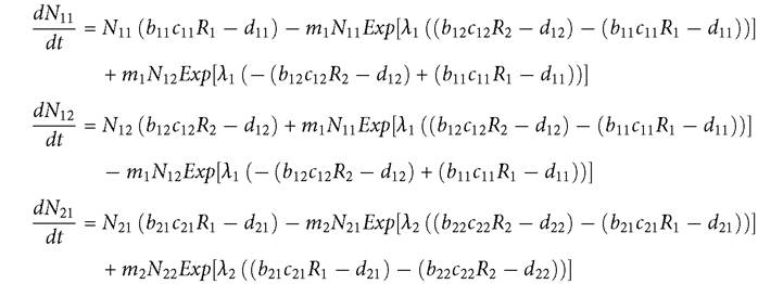
If each species is superior (has a lower R*) in a different patch, the outcome is that the two consumer species are largely, but not completely segregated in space. As a result, changing a neutral parameter (here, dij) in consumer species i by the same, relatively small amount in both patches, has little effect on the other consumer species; they retain their spatial separation, and the altered consumer decreases when its death rate is increased.
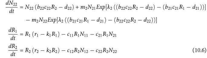
Given very accurate habitat selection (very small m and large λ) this means that, as both d2j values are increased, the abundance of species 2 will decrease in both patches, but most of this decrease is in patch 2, where almost all individuals of consumer 2 are located. Species 1 will be nearly unaffected, since it is very rare in patch 2. However, if both d2j values are increased sufficiently, d22 will pass a threshold value where species 1 becomes the superior competitor in patch 2. At that point, consumer 2 goes extinct, and consumer 1 achieves a high abundance in patch 2. The increase in species 1 caused by this disappearance may be significantly larger than the original population size of consumer 1 when both species originally have equal population sizes. This will be the case when the species differ in which patch they consume resources at a higher rate, and the consumers over-exploit the resource in their ‘preferred’ patch (equilibrium R < r∕(2k)). If so, the facts that cij < cii and that the resource growth parameters are equivalent in the two patches imply that, following the loss of consumer 2, the population of consumer 1 in patch 2 will exceed that in patch 1.In the generic case, there is some movement even when it is disadvantageous. This low level of misdirected movement is expected in natural systems due to errors in estimating resource abundances. Errors are particularly likely to characterize estimates of resources in the patch that is not currently occupied by the estimator. These errors (implied by the random movement component of eq. (10.5)) alter the consequences of mortality perturbations to either of the consumers. The effects of mortality perturbations of different sizes are described for both consumers in Figure 10.3A; this example has relatively accurate movement with m = 0.25 and λ = 10. The two consumers initially have mortality rates of d = 1 in both patches, and each has double the c-value in its initially ‘preferred’ patch compared to the ‘non-preferred’ one. The figure shows how the total population of each species changes as the per capita mortality of consumer 2 in both patches is increased by the amount given on the x-axis. In contrast to the idealized system described in the previous paragraph, there are some competitive effects at mortality rates lower than that which makes consumer 1 the superior competitor in patch 2.
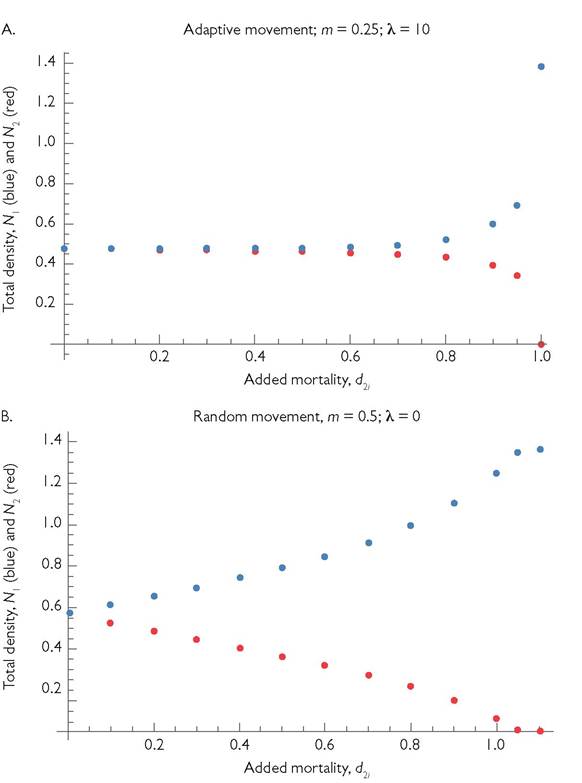
Fig. 10.3 'The competitive interaction between two mobile consumers of a single type of resource that is present in both patches, but cannot move between them. Each of the consumers has an advantage in a different patch. The dynamics within a patch are given by the MacArthurmodel, and the adaptive movement of consumers is based on eq. (10.5). The parameter values for the starting condition of consumer equality are: b11 = b12 = b21 = b22 = 1; c11 = c22 = 2; C21 = C12 = 1; d11 = d22 = d12 = d21 = 1; H = r2 = 1; and k1 = k2 = 0.1. In panel A, movement is adaptive with parameters: m1 = m2 = 0.25; and λ1 = λ2 = 10. In panel B, movement is random, with parameters: m1 = m2 = 0.5; and λ1 = λ2 = 0.
The approximately three-fold increase in the abundance of consumer 1, which follows quasi-extinction of consumer 2, occurs because the resource in patch 1 is overexploited by consumer 1. Consumer 1's lower per capita consumption rate in patch 2 produces a higher, rather than a lower, population size than in patch 1, where it captures resources more rapidly. The pattern shown in Figure 10.3A should be compared to the corresponding case of spatial competition with purely random movement. Figure 10.3B shows such a case where the random movement parameter, m, is double that in panel A. The interaction is still nonlinear, with increasing competitive effects of a fixed increase in d as the initial d becomes larger. A very unequal coexistence is possible even when consumer 2 is inferior in both patches in isolation (e.g., if it has an added mortality of 1.05). This is a result of random movement reducing the abundance of consumer 1 in patch 2, where it is more abundant.
The two consumers may differ in parameters other than c, or in multiple parameters. In all cases, the general pattern shown in Figure 10.3A still applies; uniform, fitness-decreasing changes in the parameters of one consumer will initially have small effects on the other consumer, until the species are close to competitive equality in the patch that is initially better for the manipulated species. At this point, the manipulated species decreases to extinction and its competitor increases rapidly over a relatively narrow range of the manipulated parameter. If the Figure 10.3 example were based on competitors each having a higher b value in a different patch, there would only be a two-fold, rather than a three-fold, increase in the non-perturbed consumer when its competitor became extinct in the system. If the model is modified to have abiotic resources, overexploitation is impossible, again producing smaller changes following extinction of one species. Finally, if eqs (10.6) are modified to have two resource types per patch, coexistence within an isolated patch becomes possible. However, if conditions favour a different consumer in each patch, that coexistence will involve unequal abundances, and adaptive patch movement will produce a similar (but smaller) jump in the density of one consumer when the other consumer becomes extinct.
The above treatment is far from a complete analysis, even of the simple case described by eqs (10.6). A variety of other phenomena occur with different parameter values in that model. However, the example is sufficient to show that competitive interactions in a metapopulation based on the simple MacArthur system with adaptive consumer movement have nonlinear responses quite different from those in the corresponding non-spatial (single patch) system, or a system with random movement. Having minimal spatial overlap in the original system does not imply a lack of competitive effects. The response to uniform changes in density-independent mortality is highly nonlinear, unlike those in an analogous system having differences in resource use within a single patch.
10.5.3 Adaptive movement by the resource
Another possibility is adaptive movement of the resource only, assuming spatially separated consumers. Adaptive movement should often characterize mobile biotic resources, and it might be expected to lead to nearly equal resource fitness in each patch, as predicted by ‘ideal free distribution' theory. An increase in the per capita mortality rate of one consumer (say consumer 2) will initially lower its population size, which in the short term produces an increase in the within-patch growth rate of the resource population in patch 2 plus an adaptive movement of resources from patch 1 to patch 2. The movement to patch 2 causes a decrease in the resource abundance in patch 1, which lowers the population of consumer 1. However, in the longer term, both resource populations attain new equilibria, with more resource in patch 2. The effects on the consumer may be seen by again considering a MacArthur system, this time with two patch-restricted consumers and an adaptively moving resource:
The equilibrium resource abundances are determined by the two consumer equations in eqs (10.7), unless one consumer has a death rate that is too high for that consumer to exist. The consumer abundances are determined by the resource equations. If the movement had perfect accuracy, there would be no long-term effect of changing the per capita mortality, d, of one consumer on the abundance of the other. When d2 is high enough to eliminate consumer 2, the resource in patch 2 will approach its carrying capacity. This entails a per capita resource growth rate of close to zero, which is the same growth rate of the resource at equilibrium with consumer 1 in patch 1. Using the movement function in eqs (10.7), the parameter λ must be quite large and m must be quite small to approach zero competitive effect. Otherwise, the random component of movement means that the larger resource population in the patch having few or no consumers effectively fertilizes resource growth in the other patch, leading to a slight increase in the population of consumer 1 in patch 1 when consumer 2 is reduced to zero. The generalization about small competitive effects can be confirmed by examining cases with parameters similar to the adaptive consumer example in the previous section. Purely random resource movement increases competition greatly compared to the zero-competition baseline with no resource movement. However, sufficiently accurate adaptive movement again comes close to eliminating competition at equilibrium when each of the two consumers does better in a different patch. These results have some similarities to a single-patch system in which the resource exhibits adaptive defence with a linear trade-off between avoiding/defending against one or the other type of predator (Matsuda et al. 1993).
10.6
More on the topic Adaptive movements and their effects on competition:
- 11.l Evolution’s many effects on interspecific competition
- Moral Permissibility as a Product of Effects Over Time, Not Momentary Effects
- Adaptive Interfaces
- Adaptive Equipment
- Adaptive Behavior
- The Size and Distribution of the Movements
- Adaptive Evolution
- What are the Causes of these Movements?
- Adaptive Sports and Recreation
- Adaptive movement of both species
- Resistance Movements and Social Justice
- Adaptive evolution can occur rapidly