INEQUALITY: TRENDS

In this section we report the recent trends in income inequality in the developing coun­tries. We start laying out the general patterns, and then dig deep into the evidence for each region.

9.4.1 General Changes

The available evidence suggests that on average the levels of national income inequality in the developing world increased in the 1980s and 1990s and declined in the 2000s. Using data from PovcalNet, the mean Gini for the distribution of per capita consumption

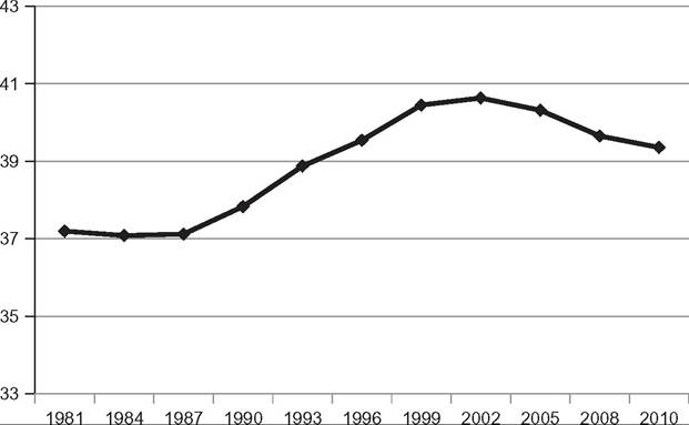
Figure 9.5 Gini coefficient. Unweighted mean for developing countries, 1981-2010. Note: The national Gini coefficients are computed over the distribution of household consumption per capita. Source: Own calculations based on PovcalNet (2013).

expenditures increased from 37.2 in 1981 to 39.4 in 2010 (Figure 9.5). ^[485] The mean was basically unchanged between 1981 and 1987,^[486] then increased more than three points to reach a value of 40.5 in 1999, and from 2002 it started to fall, although slowly (from 40.6 in 2002 to 39.4 in 2010).^[487]

Figure 9.6 adds to the picture the changes at different percentiles of the distribution of national Ginis. The figure makes clear that on average the changes in the last decades have not been large compared to the range over which the Gini varies across countries.^[488] The picture also reveals that the growth in the mean Gini in the late 1980s and 1990s

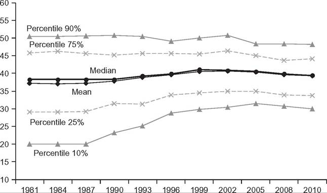
Figure 9.6 Distribution of Gini coefficients.

was mainly due to the substantial increase in the low-inequality countries, in particular Eastern Europe and Central Asia economies after the fall of communism, and also some Asian economies in the early stage of economic takeoff.Instead, the fall in the 2000s was widespread, although more intense in those countries above the median, such as those in Latin America. This observation suggests convergence in the levels of inequality in the developing economies. In fact, the standard deviation for the distribution of Gini coef­ficients substantially fell over time: 11.2 in 1981, 10.1 in 1990, 7.4 in 1999, and 7.2 in 2010. Countries in the developing world are still very different in terms of income inequality, but differences have become considerably smaller over the last three decades (more on convergence below).

A closer inspection of the data reveals that the result of a stable mean Gini in most of the 1980s is driven by the lack of information for several countries and by a substantial heterogeneity in the changes of those with information (Table 9.7).^[489] The strong rise in the mean Gini in the 1990s is associated with a large proportion of countries with grow­ing inequality in a framework of much improved information. The tide seems to have turned in the 2000s, when most of the countries in the sample experienced a fall in

Table 9.7 Proportion of countries classified in groups according to the change in the Gini coefficient

1981-1990 1990-2002 2002-2010

Note: “Fall” includes countries where the Gini fell more than 2.5% in the period; “Increase” includes countries where the Gini rose more than 2.5%; “No change” includes countries where the Gini changed less than 2.5%; “No information” includes countries without two independent observations in each period.

Source: Own calculations based on PovcalNet (2013).

inequality. But even in this decade of widespread social improvement, the country per­formances in terms of inequality reduction were quite heterogeneous. In fact, in 20% of the economies of the developing world the Gini coefficient increased between 2002 and 2010, whereas in 15% of the countries the changes were smaller than 2.5%.

We find that the bulk of the countries in the sample (62%) experienced a change in the pattern of inequality around the turn of the century, from nonfalling to decreasing inequality, whereas only a few experienced a pattern of continuous increasing (15%) or decreasing (12%) disparities. In fact, an inverse-U shape for the inequality pattern is observed for many economies (45% of the sample), a fact that could be consistent with the Kuznets story of economic growth for countries located close to the curve turning point. However, we fail to find any significant correlation between the type of the inequality pattern and different measures of development and growth. The inverse-U pat­tern in the period 1981—2010 appears to have been common to a wide range of economies.

The growth in the population-weighted mean of the Gini coefficient across devel­oping countries was stronger than the increase in the unweighted mean (Figure 9.7). Although the latter increased 2.2 points in the period 1981—2010, the former jumped

7.5 points. The gap between the two means shrunk from 5.4 points in the early 1980s to almost zero in the late 2000s. This pattern is mainly accounted for by the dra­matic surge in income inequality in China over the period. Interestingly, the fall in the unweighted mean Gini in the 2000s does not show up in the weighted mean; although the Gini coefficient for a typical developing country significantly decreased in the 2000s, the national Gini for a typical person in the developing world did not fall.

In the rest of this section we go beyond the Gini coefficient and track changes along the distribution.

44

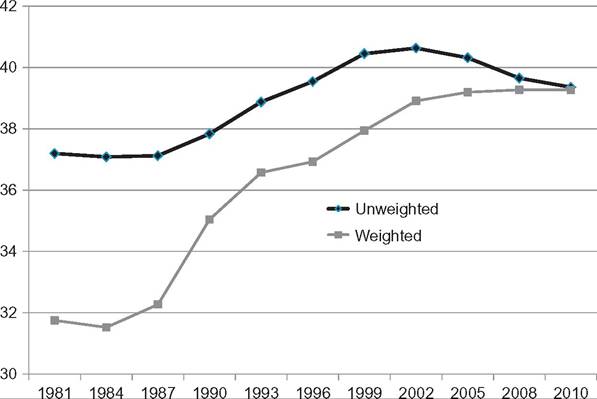
Figure 9.7 Gini coefficient. Weighted and unweighted means. Developing countries, 1981-2010. Note: The Gini coefficients are computed over the distribution of household consumption per capita. Source: Own calculations based on PovcalNet (2013).

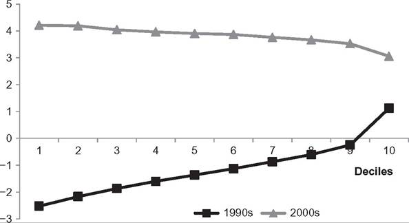
Figure 9.8 Growth-incidence curves. Annualized growth rate in consumption per capita by decile. Unweighted mean for developing countries. Note: Annual change in consumption per capita (PPP US$). 1990s ¼ 1990-2002, 2000s ¼ 2002-2010. Source: Own estimates based on PovcalNet (2013).

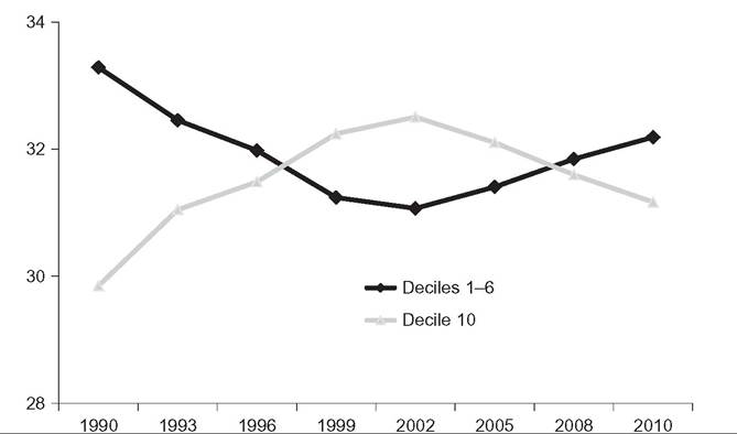
Figure 9.9 Decile shares. Unweighted mean for developing countries, 1990-2010. Note: The decile shares are computed over the distribution of household consumption per capita. Source: Own estimates based on PovcalNet (2013).

contrast in the GIC corresponding to the 1990s and the 2000s. The first one is clearly increasing, suggesting growing inequalities, whereas the second is decreasing (and flatter), indicating a fall in well-being disparities in the 2000s. On average, in that decade con­sumption per capita grew by more than annual 4% in the three bottom deciles of the national distributions and by 3% in the top decile.

Naturally, the contrast between decades is also evident when looking at income shares. The results are summarized in Figure 9.9: whereas the share of the bottom 60% fell 2 points in the 1990s and increased 0.9 points in the 2000s, the performance of the top 10% was almost the exact mirror.

9.4.2 Changes by Region

Changes in inequality have been heterogeneous across the six geographical regions of the developing world (Figure 9.10).^[491] The mean Gini coefficient in Latin America increased more than two points in the 1990s and then dropped in the 2000s by a larger amount. The data reveals almost no change in inequality in sub-Saharan Africa over the two last

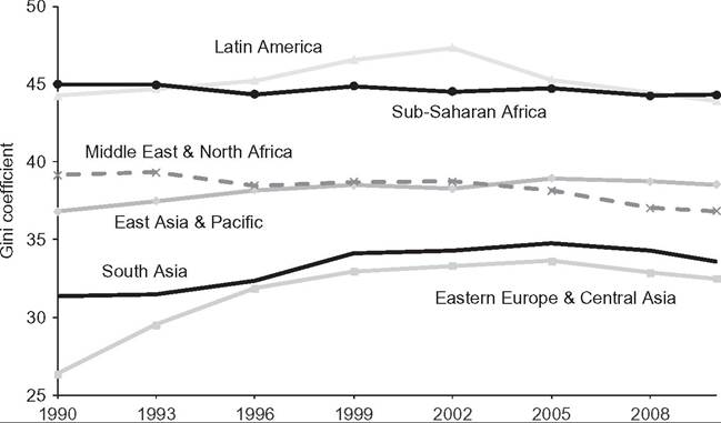
Figure 9.10 Gini coefficients. Unweighted means by region, 1990-2010. Note: The Gini coefficients are computed over the distribution of household consumption per capita. Source: Own estimates based on PovcalNet (2013).

decades and some decline in the five MENA countries included in the sample. Instead, the Gini coefficient increased more than two points in Asia and more than six points in Eastern Europe and Central Asia. Figure 9.10 suggests again some pattern toward con­vergence; the gaps in inequality among regions in the developing world are smaller now than two decades ago. For instance, whereas the gap in the Gini coefficient between Latin America and ECA was 18 points in the early 1990s, it shrank to 11 points in the late 2000s.

In all the regions the share of countries with falling inequality rose in the 2000s, as compared to the 1990s. The two most remarkable changes in the pattern occurred in Latin America and in Eastern Europe and Central Asia. Whereas the Gini went down in 26% of the LA economies in the 1990s, that share increased to 95% in the 2000s. In ECA, whereas the growth in inequality was generalized in the 1990s, more than half of the countries experienced reductions in the 2000s.

Using data from PovcalNet, Chen and Ravallion (2012) report changes in the within component of the global mean-log deviation between 1981 and 2008.

The picture of national inequalities in the developing world is similar when using other databases. For instance, the unweighted mean Gini in the All the Ginis database assembled by Milanovic grew from 36.2 in 1990 to 40.7 in 1999 and then dropped to 39.7 by 2005. Whereas in the 1990s inequality rose in 63% of the economies in the ATG database, that share dropped to 35% in the 2000s. The recorded increase in the 1990s was generalized across regions, but especially intense in Eastern Europe and Central Asia (9 Gini points), whereas the fall in the 2000s was larger in MENA and Latin America. CorniaandKiiski (2001), Cornia (2011), and Dhongde and Miao (2013) document sim­ilar results using WIID data. We find that the linear (rank) correlation coefficient for the change in the Gini coefficient between 1990 and 2005 recorded in PovcalNet and WIID is 0.776 (0.868), significant at 1%. The corresponding values forthe comparison between PovcalNet and ATG are 0.721 and 0.765.

The evidence drawn from the EHII database is also roughly consistent with the pat­terns discussed earlier. The mean Gini for the developing world remained almost unchanged in the 1980s, increased in the 1990s from 42.5 in 1990 to 47.0 in 1999, and dropped to 46.5 in 2002 (the latest available date).^[492] Whereas in 62% ofthe countries inequality increased in the early 1990s, that share dropped to 55% between 1993 and 1999 and to 49% between 1999 and 2002. The regional patterns are roughly consistent with those described earlier. The main difference is that EHII reveals a dramatic increase in inequality in the Middle East and North Africa (7 Gini points) that is not present in the evidence drawn from household surveys.

In the rest of this section we briefly review the literature on inequality changes in each geographic region of the developing world, while we take a closer look to the story of some particular cases: Brazil, China, India, Indonesia, and South Africa.

9.4.2.1 East Asia and Pacific

The inequality patterns in East Asia and Pacific can be traced based on information from only 8 out of the 24 countries in the region, which nonetheless represent 96% of its total population. This set includes Cambodia, China, Indonesia, Lao PDR, Malaysia, Philippines, Thailand, and Vietnam. There is scattered evidence for Fiji, Micronesia, Mongolia, and Timor-Leste, but information is either lacking or too scarce for American Samoa, Kiribati, Korea, Dem. Rep., Marshall Islands, Myanmar, Palau, Papua New Guinea, Samoa, Solomon Islands, Tonga, Tuvalu, and Vanuatu.

The slightly increasing pattern showed in Figure 9.10 for the unweighted mean of the consumption Gini in EAP hides important differences across countries (ADB, 2012; Chusseau and Hellier, 2012; Ravallion and Chen, 2007; Sharma et al., 2011; Solt, 2009; Zin, 2005). Consumption inequality increased in most economies in the region during the 1990s, with the exception of Thailand and Malaysia. The increase was

particularly strong in China, where the consumption Gini climbed around seven points in that decade. The performance in the 2000s was more heterogeneous; inequality con­tinued increasing in China, Lao PDR, and Indonesia and also went up in Malaysia, but there is evidence pointing to a fall in consumption inequality in Cambodia, Philippines, Thailand, and Vietnam.

Overall, considering the two decades, EAP combines countries with systematic increases in inequality (China, Indonesia, Lao PDR), several cases in which inequality had a cyclical pattern, ending in 2010 at similar levels than in 1990 (Cambodia, Malaysia, Philippines, and Vietnam), and only one successful story of consistent reduction in con­sumption inequality: Thailand, for which the estimated reduction in the Gini coefficient exceeded five points; from 45.3 to 39.4 over the last two decades. Universal social pol­icies, including basic education and health, have been stressed by many authors as signif­icant drivers of that fall (Jomo and Baudot, 2007).

Probably the most striking phenomenon regarding inequality in EAP was the strong rise that took place in the two most populous countries of the region, China and Indonesia: the Gini coefficient went up around 5 points in Indonesia and more than 10 points in China over the last two decades. Such dynamics happened in a context of high growth and falling poverty, most notably in China. Sharma et al. (2011) summarize the main fac­tors behind these changes: (i) the realignment of activity away from agriculture and toward industry and services; (ii) the skill premium increase due to the unmatched growing demand for skills, and even the emigration of skilled workers; (iii) increasing inequalities in educational attainment in secondary and tertiary schooling; and (iv) a lack of infrastruc­ture linking urban areas with rural areas and other barriers to labor mobility.

rural-urban divide in employment and earning possibilities, exacerbated by the much more rapid development that occurred in coastal areas. Interestingly, in marked contrast to most developing countries, relative inequality is higher in China’s rural areas than in urban areas. However, there has been convergence over time with a steeper increase in inequality in cities.

Indonesia

During the 30 years before the Asian crisis of 1997-1998, which coincided with the New Order under Suharto’s dictatorship, Indonesia GDP grew at an average rate of 7% per year. The process was not smooth and went through different phases that implied immense structural change. Despite problems with the data, scholars agree in that there was a systematic drop in poverty rates between 1976 and 1997. At the same time, overall consumption inequality in Indonesia did not change markedly with development until the late 1980s, when inequality started to rise, driven by increasing income disparities in urban areas. Alatas and Bourguignon (2000) decompose the inequality increase between components associated with changes in the structure of earnings, changes in occupational choice, and changes in the sociodemographic structure of the population. They find as main explanations the migration from rural to urban areas and the increase in nonfarm self-employed work. The increase in inequality was partly offset by shrinking income gaps in rural areas (Cameron, 2002). Alatas and Bourguignon (2000) find that the returns to land size decreased between 1980 and 1996; opportunities for off-farm earnings for rural households also contributed to falling rural inequality.

Indonesia was severely hit by a financial crisis: In 1997-1998 GDP dropped by 15%. This turned into a sharp decrease in inequality and an increase in poverty. Skoufias and Suryahadi (2000) find that this pattern seems to have arisen from a decrease in regional inequality. Urban areas (which tend to be wealthier than neighboring rural areas) were hit harder, and the urban middle class, who lost their formal sector jobs, was harshly affected. As the crisis reduced the per capita expenditure of households, the percentage reduction was probably less among the poorer population than among the less poor population. Since 2001, and along with the process of decentralization of powers to local authorities, a general pattern of rising consumption inequality has been observed. Miranti et al. (2013) suggest that the recent increases in inequality may be linked to the higher share of workers employed in the informal sector (70%), hence not covered by minimum wage legislation or employment protections.

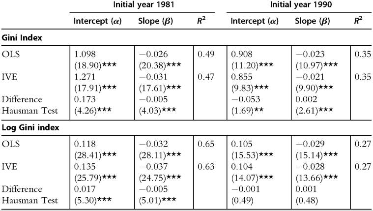
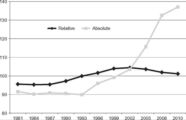
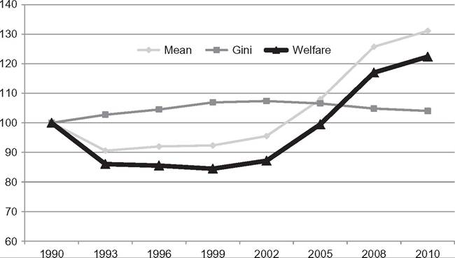
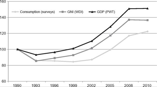
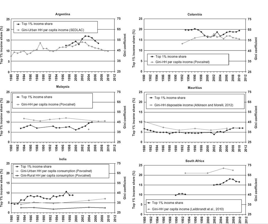
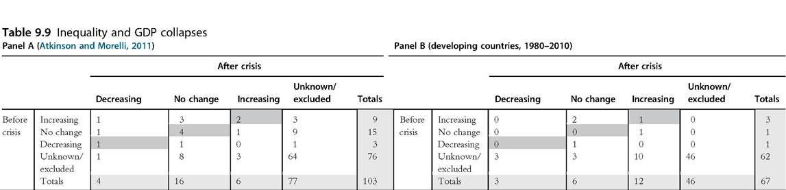
administrations (Milanovic, 1998).^[493] The fall of the communist regimes was followed by a substantial increase in inequality in almost all countries.^{[494] [495] [496] According to PovcalNet data the mean Gini for the distribution of per capita consumption expenditures grew from 26.4 in 1990 to 31.9 in 1996. The increase in the first half of the 1990s was particularly strong in those countries belonging to the FSU and in Southeast Europe and somewhat milder in those economies that joined the European Union. Such developments have been linked to the process ofprivatization, which implied an increase in earnings dispersion in compar­ison to the more compressed wage structure of the state-owned firms. One key character­istic of the planned economies was the imposition of wage “grids” that forced a wage compression; the fast transition from wage setting under the wage grids toward a less- regulated labor market provoked a rise in the returns to education, and hence a surge in inequality. , 0 The economic liberalization also triggered changes in the sectorial structure of the economy; in particular the ensuing de-industrialization during the transition is linked to an increase in inequality (Birdsall and Nellis, 2003; Ferreira, 1999; Ivaschenko, 2002; Milanovic, 1999). Milanovic and Ersado (2010) highlight the role played by the inception or increase of tariffs for utilities, whereas Standing and Vaughan-Whitehead (1995) point to the weakening of the minimum wage as key factors behind the increase in inequality.}

After the initial surge in the early 1990s, inequality continued growing in the region in the second half of the 1990s although at slower rates. The patterns were more hetero­geneous in the 2000s; inequality increased in some economies, but went down in most countries, especially those in the FSU (World Bank, 2005). The mean Gini for Eastern Europe and Central Asia in the late 2000s was lower than in the late 1990s but still significantly higher (around 7 Gini points) than before the transition.^[497]

9.4.2.3 Latin America and the Caribbean

All Latin American countries regularly carry out national household surveys that include income questions, and in some of them also questions on consumption expenditures.^[498] In contrast, the situation in the Caribbean is much less favorable, as surveys are sporadic, and information is not easy to access. In fact, trends shown in the literature and in this section are restricted to Latin America, which represents 94% of total LAC population.

Latin America experienced two distinct distributive patterns in the last three decades (De Ferranti et al., 2004; Gasparini et al., 2011a,b; IDB, 1999; Lopez Calva and Lustig, 2010). Duringthe 1980s, 1990s, and the crises at the turn of the century, income inequal­ity soared in most countries for which comparable data are available. The mean Gini for the distribution of household per capita income crawled from 50.1 in 1980 to 51.5 in 1986, 51.9 in 1992, 53.0 in 1998, and 53.4 in 2002 (Gasparini et al., 2013). The frequent macroeconomic crises that hit the region in that period were unequalizing because the poor were less able to protect themselves from high and runaway inflation, and adjust­ments programs frequently hurt the poor and the middle-class disproportionately (Lustig, 1995). The market-oriented reforms that started in Chile in the 1970s and became wide­spread in the region in the 1990s were associated with rising inequality, although this pattern had a notable exception in the case of Brazil (Lopez Calva and Lustig, 2010). In most countries employment reallocations brought about by trade liberalization and the skilled-biased technical change associated to the modernization of the economy implied a sizeable reduction in the demand for unskilled labor, which led to higher inequality. In some countries adjustments that led to a contraction in the demand for labor affected unskilled workers disproportionately. All these changes took place in a framework of weak labor institutions and safety nets, and hence their consequences made a full impact on the social situation (Gasparini and Lustig, 2011).

Starting in the late 1990s in a few countries and in the early 2000s for the rest, inequal­ity began to decline. The mean Gini for the distribution of household per capita income dropped from 53.4 in 2002 to 50.9 in 2008 (Gasparini et al., 2013). Updated SEDLAC and BADEINSO statistics suggest that the downward trend continued. The evidence, in fact, indicates that between 2002 and 2013 income inequality went down in all Latin American economies. This remarkable decline appears to be driven by a large set of fac­tors, including the improved macroeconomic conditions that fostered employment, the petering out of the unequalizing effects of the reforms in the 1990s, the expansion of coverage in basic education, stronger labor institutions, the recovery of some countries from severe unequalizing crises, and a more progressive allocation of government spend­ing, in particular monetary transfers. The empirical evidence on the driving factors of the recent fall in inequality is, however, still scarce and fragmentary (Cornia, 2011; Gasparini and Lustig, 2011; Lopez Calva and Lustig, 2010).

from that point on inequality started to decrease, first slowly in the 1990s, and then more dramatically in the 2000s. By 2011 the Gini reached an unprecedented low value of 52.7, several points below the level of some other Latin American economies (e.g., Honduras, Colombia, Bolivia).^{[499] [500] [501] [502] Brazil—the fifth most populous nation in the world—is still a high-inequality country, but it stands out as a successful case of consistent reduction of income disparities.}

Data from the Brazil's national household survey (PNAD) reveals a drop in the Gini of 2 points in the late 1970s and no systematic changes for most of the 1980s, until a deep macroeconomic crisis hit the country, pulling inequality to unprecedented levels. The Gini went up from 59.2 in 1986 to 62.8 in 1989 and returned to 59.9 in 1993. During the 1990s the Gini moved down very slowly, decreasing by just 1 point between 1993 and 2001. That pace drastically increased in the 2000s: the Gini went down from 58.8 in 2001 to 52.7 in 2011, averaging a fall of 0.6 points a year. During 10 years per capita income of the poorest 10% of the Brazilian population grew at an average annual rate of 7%, almost three times the national average.

In an in-depth study of the determinants of inequality changes in Brazil, Barros et al. (2010) highlight the role played by the sharp fall in earnings inequality and the substantial increase in public transfers as the two main direct determinants of the decline in income disparities since the early 2000s.⁵ They find that half of the reduction of inequality in labor incomes was associated to the educational progress that took place over the previous decade, which significantly increased the ratio between skilled and unskilled workers. The average years of education for the adult population grew 22% in the 2000s, and the Gini coefficient computed over the distribution of that variable fell 23%, values well above the mean for Latin America (Cruces et al., 2014). Using different decomposition techniques, Barros et al. (2010) and Azevedo et al. (2011) find a sizeable impact of the fall in the returns to education on earnings inequality. Several authors have also found a reduction in spatial and sectorial labor market segmentation. The substantial increase in the minimum wage—68% in real terms between 2002 and 2010—is also underlined as one important force behind the fall in household income inequality, given that the minimum wage sets the floor for both unskilled workers earnings and for social security benefits.

The strong expansion of public transfers accounts to a large share of the fall in income inequality in Brazil (Azevedo et al., 2011; Barros et al., 2010; Alejo et al., 2013; Lustig et al., 2012). The main force was the rapid expansion in the coverage of government cash transfers targeted to the poor, mainly a transfer to the elderly and disabled (Beneficio de Prestafeio Continuada) and Brazil’s signature conditional cash transfer program Bolsa Familia.

53

54

55

56

9.4.2.4 Middle East and North Africa

Data constraints are particularly Iimitingwhen analyzing distributive issues in Middle East and North Africa. The lack of accessible and comparable household surveys makes it difficult even to identify the extent of poverty and inequality in most MENA countries. The oil-rich economies (Bahrain, Kuwait, Oman, Qatar, United Arab Emirates, and Saudi Arabia) enjoy high levels of per capita income and are usually not included in the analysis of the developing world. In any case, distributive data is rarely available for these economies. A second group, by far the largest in terms of population, consists of middle-income countries. Within this group there is no public accessible information for Lebanon and Libya, just one data point for Djibouti, Iraq, Syrian Arab Republic, West Bank, and Gaza, and only a few for Algeria and Yemen. In sum, the only MENA coun­tries for which it is possible to track changes in poverty and inequality over time are Egypt, Iran, Jordan, Morocco, and Tunisia, but even in these cases data is scattered and often of low quality. MENA has a long way to go to build a reliable, comparable, and sustainable system of household surveys and distributive statistics.

Despite this constraint, several studies shed some light on the trends in inequality in this region.^[503] Authors coincide in dividing the last four decades into three periods. The first one, spanning until 1985, was characterized by rapid economic growth. Page (2007) reports a substantial reduction in income inequality between the mid-1970s and the early 1990s.^{[504] [505] Data from PovcalNet confirms that fall, although the magnitude is more modest. “Middle Eastern economies entered their rapid growth period with income distributions that were becoming more egalitarian, reflecting the political ideology and policies of post-colonial governments” (Page, 2007). The second period covers the late 1980s and most of the 1990s and is characterized by low economic growth and meager or no social gains; real per capita incomes increased by less than 1.5% per year, whereas income distributions were rather stable. The downward pattern in inequality appeared to have resumed in the 2000s, although at a slow pace. According to our estimates based on PovcalNet, the mean Gini fell from 38.7 in 2002 to 36.8 in 2010. These values place MENA as a region of moderate inequality within the developing world, a fact that has puzzled some authors, that would predict higher income disparities given the political process and the balance of political power in those societies.5}

Alvaredo and Piketty (2014) analyze the issue from a regional perspective and show that, irrespective of the uncertainties on within-country disparities, income inequality is extremely large at the level of the Middle East taken as a whole, simply because regional inequality in per capita GNP is particularly large. Under plausible assumptions, the top 10% income share could be well over 60%, and the top 1% share might exceed 25% (vs. 20% in the United States, 9% in Western Europe, and 18% in South Africa). The authors conclude that the popular discontent that contributed to the Arab spring revolt might reflect the fact that perceptions about inequality and the (un)fairness of the distri­bution are determined by regional (and/or global) inequality, and not only on national inequality.

9.4.2.5 South Asia

South Asia has been a region of low inequality for developing world standards, though rising since the early 1990s. In India, further discussed in a separate box, the consumption Gini moved from 30.8 in 1993 to 33.9 in 2010. Bangladesh displayed relatively low inequality throughout the 1980s (Gini equal to 26.1 in 1984), but the situation worsened since the beginning ofthe 1990s: the Gini climbed to 32.1 by 2010. Khan (2008) argues that incomes from nonfarm sources and the high concentration of land tenure have all been disequalizing forces, whereas the positive effects of the more-evenly distributed farm income were offset partly by its declining share in total income.

Scholars do not always agree about the distributive changes in Pakistan; PovcalNet helps defining the picture by providing consumption Ginis of 33.2 for 1990, 28.7 for 1996 and 30.0 for 2008. The high economic growth during the 1980s contributed to a sharp decline in poverty, but it was accompanied by a mild increase in inequality. The fall in economic growth during the 1990s resulted in a rise in poverty, whereas inequality decreased modestly. According to Hussain (2008) in Pakistan there is an insti­tutional structure that excludes a large proportion of the population from the process of economic growth as well as governance.

Sri Lanka experienced rising inequalities between 1985 (Gini of 32.5) and 2007 (Gini 40.3)—among the highest increase in the region during the period of free market reforms, integration to the world markets and high growth—with a reversal ofthe trend toward 2010 (Gini of 38.3) and persistent regional disparities due to conflict. Nepal pre­sents similar dynamics. Gosh (2012) notes that rising inequality reflects two components: first, growing vertical inequality within the modern industrial sector driven by the returns to skill, and second, increasing disparities between the industrial fast-growing sector and the traditional agricultural activities.

India

Chakravarty (1987) argues that even if policymakers in India adopted a development strategy based on central planning over the 40 years following independence, “there was a tolerance towards income inequality, provided it was not excessive and could be seen to result in a higher rate of growth than would be possible otherwise.” One of the explicit goals of the socialist program was to limit the economic power of the elite in the context of a mixed economy. From the mid-1980s, however, India gradually adopted market-oriented economic reforms. Initially, these were accompanied by an expansionist fiscal policy involving allocations to rural areas, to counterbalance the negative redistributive effects of the liberalization. The speed of reforms accelerated during the early 1990s, and the focus shifted away from state intervention toward liberalization, privatization, and globalization.

Most analysis on inequality in India over the last three decades are based on the observations from the expenditure surveys conducted in 1983, 1987/8, 1993/94, 2004/05, and 2009/10 for urban and rural areas, which have allowed for an analysis pre- and postreforms. Inequality increased significantly in the postliberalization years, especially in urban areas; on the contrary, estimates of absolute poverty measures have systematically fallen since 1983. Mazundar (2012) summarize the main drivers of these changes: (i) the lead in employment and output growth has been taken not by manufacturing but by the tertiary sector, which displays higher inequality in pay; (ii) much of the labor reallocated from agriculture is absorbed in the informal sector, where earnings are only slightly higher than the poverty line; (iii) although numerous social insurance schemes have been established, their actual impact has been limited and regressive as they have disproportionately benefited workers in the small formal sector; (iv) the modest and selective increase in social sector spending is constantly threatened by the budget deficit; (v) the education polices implemented over the years have been biased toward the promotion of tertiary education and have neglected basic primary and lower secondary education.

From a different perspective, Banerjee and Piketty (2010) look at the tax-based shares of top incomes. Their results suggest that the gradual liberalization of the Indian economy made it possible for the top 1% to substantially increase their share of total income, from 4.7% in 1980 to 8.9% in 1999. Although in the 1980s the gains were shared by everyone in the top percentile, in the 1990s it was those in the top 0.1% who benefited the most.^[506]

SSA countries are missing (Equatorial Guinea, Eritrea, Mauritius, Somalia, Zimbabwe), whereas for 13 of them there is only one observation in the database for the whole period 1981—2010. In fact, very few countries have reliable surveys in the 1980s, and it was not until the mid-1990s when inequality could be really traced with some confidence in the region.

Regional studies typically report a mixed picture, with both increases and decreases in inequality, a fact that could reflect the heterogeneity in the region, but also could be caused by noise in the country estimations (Christiansen et al., 2002; Okojie and Shimeles, 2006). Bigsten and Shimeles (2003), for instance, report that for 17 African countries the trend in inequality shows significant variations over short periods, causing concern about measurement problems.

The available evidence seems to support some few broad facts about consumption inequality in the sub-Saharan African countries. First, inequality is very high on average, possibly the highest in the world. This result is in stark contrast with the presumption of low inequality in SSA, held for a long time based on the predictions of Kuznets-like models and the absence of reliable data.^{[507] [508] [509] Second, on average inequality does not seem to have changed much in the 1990s and 2000s. Data from PovcalNet and other sources suggest a slow downward pattern; but in any case the evidence is mixed and weak. Third, the heterogeneity among countries in terms of inequality levels and patterns is large, partly possibly due to various measurement errors. It is hard to identify a prototype of an inequality pattern in SSA, as in other regions such as LAC or ECA. The scarce liter­ature on inequality in SSA is consistent with these observations. Go et al. (2007) report that high income inequality levels in SSA have remained more or less constant over the last four decades. Okojie and Shimeles (2006) underline the fact that SSA is one of the most unequal regions in the world, and that disparities have remained persistent over time. In contrast, Sala-i-Martin and Pinkovskiy (2010) picture a more optimistic sce­nario, reporting a significant downward pattern for inequality during the period of growth (1995-2006).}

with this view, the country has the highest Gini coefficient of household consumption per capita (63.1 in 2010). During the early 1970s, the previously constant racial shares of income started to change in favor of the blacks, at the expense of the whites, in a context of declining per capita incomes (McGrath, 1983; McGrath and Whiteford, 1994). But while interracial inequality fell throughout the eighties and nineties, inequality within race groups increased (Simkins, 1991; Whiteford and Van Seventer, 2000). Leibbrandt et al. (2010a, 2010b) provide evidence from comparable households’ surveys conducted in 1993, 2000, and 2008. These authors find that since the fall of apartheid, inequality continued to increase steadily, both for the whole population and within each racial group. The high level of overall income inequality accentuated between 1993 and 2008, incomes becoming increasingly concentrated in the top decile. van der Berg and Louw (2004) also conclude that rising black per capita incomes over the past three decades have narrowed the interracial income gap, although increasing inequality within the black and Asian/Indian population seems to have prevented any decline in aggregate inequality.

In explaining these changes scholars agree in that the labor market played a dominant role, where a rise in the number of blacks employed in skilled jobs (including civil service and other high-paying government positions) coupled with increasing mean wages for this group of workers. Leibbrandt et al. (2010a, 2010b) indicate that in the initial post-apartheid period participation rates increased faster than absorption rates with a consequent increase in unemployment across all deciles. Since 2000 the aggregate unemployment rate declined, but the in the lower deciles the early post-apartheid trend continued to 2008. State transfers have increased their importance as an income source but not in a way that has substantially narrowed the income gaps. They have, however, compensated for the decreasing share of remittance income.

Increasing inequality and stable poverty are consistent with the rising trend in top income shares recorded between 2002 and 2010 by Alvaredo and Atkinson (2010), which could be associated with the favorable conditions in the world market for agricultural commodities, the increase in the value of minerals other than gold, and the developments in the financial sector.

9.4.3 Inequality Convergence

As suggested earlier, there are signs of inequality convergence among countries in the developing world. As an example, the mean Gini coefficient for the 20 most unequal countries in our PovcalNet sample in 1981 fell 11% in the following three decades, while it increased 58% for the 20 most egalitarian economies. Benabou (1996) was the first to present empirical evidence for cross-country convergence in income inequality with data from 1970 to 1990 drawn from the Deininger and Squire data set. He found evidence consistent with the predictions of a neoclassical growth model that yields convergence of the entire income distribution and not just the first moment.^[510] Evidence on inequality convergence was also found in studies that used improved data: Ravallion (2003) based on PovcalNet, Bleaney and Nishiyama (2003) based on WIID, and Dhongde and Miao (2013) using both data sets. With variations, a typical inequality convergence study estimates

Git - Gn = (α + βG,∙1)(f- 1) + e⅛ for t = 2,..., T; i = 1,...,N, where G_it is the Gini coefficient for country i in year t, and e_it is an heteroscedastic error term. The parameter β measures the link between the change and the initial Gini, and therefore β < 0 indicates inequality convergence. Models could be estimated with the Gini coefficient in levels or logs. In his early study Benabou (1996) found a β coefficient of —0.039 for a small sample of around 30 countries. Naturally, estimates of β vary according to the data used, the period covered, the time horizons considered, and the regression model applied. Ravallion (2003) estimated a value of —0.028 in the 1990s, Bleany and Nishiyama (2003) a value of —0.0125 between 1965 and 1990, and Dhongde and Miao (2013) a value of —0.022 from 1980 to 2005. This literature has also found that the impact of the initial Gini coefficient on the inequality change diminishes over longer time horizons, and that the speed of inequality convergence is higher than the speed of convergence in per capita income.

We add to this literature our own estimates, taking advantage of the PovcalNet panel of76 countries from 1981 to 2010 used in this section. Table 9.8 shows the OLS and IVE estimates of α andβ for different initial years.^[511] The parameter β is negative and significant in all the specifications, suggesting evidence for inequality convergence. The estimated coefficients are in the range of those estimated in the literature.

Although the evidence for inequality convergence in the last decades seems well established, the reasons driving that pattern are not clear. As mentioned before, Benabou (1996) finds the evidence on convergence consistent within the framework of a growth model. In contrast, the evidence for unconditional inequality convergence is interpreted by Ravallion (2003) as the result of policy and institutional convergence since around 1990, when socialist planned economies became more market-oriented, and non-socialist economies adopted market reforms.

Table 9.8 Inequality Convergence

Models of the change in the Gini coefficient

Note: Robust t statistics in parentheses; **significant at 5%; ***significant at 1%; the heteroskedasticity-consistent covari­ance matrix estimator is used (HC1). IVE estimates use the initial value as the instrument for the inequality measure in the second survey. The number of observations is 456 in the first panel and 281 in the second.

9.4.4 Absolute Inequality

Although relative inequality has been the preferred concept in empirical work in devel­opment economics, absolute views of inequality certainly have some intuitive appeal (Amiel and Cowell, 1999; Atkinson and Brandolini, 2004). Interestingly, the trends in the two concepts over the last decades have been different in the developing world.^[512] The fact that most countries experienced economic growth, while at the same time rel­ative inequality did not fall, implied widening absolute income differences. On average, the absolute difference in monthly consumption per capita between the top and bottom 10% of each country increased over the two decades from US$ 415 (PPP adjusted) in 1990, to US$ 497 in 2002, and US$ 646 in 2010. In more than 90% of the countries in the sample that absolute difference was higher in 2010 than in 1990.

The contrast between the recent trends in absolute and relative inequality in the developing countries is illustrated in Figure 9.11. Whereas relative inequality rose in the late 1980s and early 1990s, absolute inequality declined, driven by a reduction in

65

Figure 9.11 Absolute and relative Gini coefficients. Unweighted means, developing countries, 1981-2010. Note: Normalized to 100 ¼ mean over the period 1981-2010. The Gini coefficients are computed over the distribution of household consumption per capita. Source: Own estimates based on PovcalNet (2013).

mean income. The strong growth in the developing world since mid-1990s is reflected in the substantial hike in the degree of absolute inequality. Although some equalizing forces operated in the 2000s that reduced the relative gaps, they were not enough to narrow the absolute gaps in a context of economic growth. Based on these facts, Ravallion (2004) argues that the disagreements over whether inequality in the world has gone up or down may partly be due to differing views about the importance of absolute versus relative con­ceptions of inequality.

9.4.4 Aggregate Welfare

The typical way of assessing the economic performance of a country is by means of its per capita income or output. However, this practice is valid only when the evaluator’s wel­fare function is utilitarian. Except in this extreme case, measuring aggregate welfare involves not only knowing the mean but also other elements of the income distribution, in particular the degree of inequality. Although social welfare functions are naturally arbi­trary, because they depend on the analyst’s value judgments, it is common in the literature to work with anonymous, Paretian, symmetric, and quasiconcave functions. For

Figure 9.12 Aggregate welfare. Sen welfare function, unweighted mean, developing countries, 1990-2010. Note: Normalized to 100 = value in 1990. Source: Own estimates based on PovcalNet (2013).

simplicity, here we consider the abbreviated welfare function proposed by Sen (1976), W_s=μ(1 — G), where μ is the mean of the distribution and G is the Gini coefficient. Figure 9.12 shows the unweighted mean of W_s for the developing countries in the period 1990-2010 computed from household survey data. In general, aggregate welfare has fol­lowed changes in per capita consumption. The fall in mean consumption in the early 1990s (mostly due to the negative performance in ECA) was reinforced by the increase in inequality, driving welfare down by around 15%. Between 1993 and 2002 mean consumption went up, but the change was counterbalanced by a similar increase in the Gini, keeping welfare roughly constant. The 2000s witnessed a robust increase in mean consumption, along with some fall in inequality, implying a 40% increase in aggre­gate welfare between 2002 and 2010. According to these calculations, the mean aggregate welfare in the developing countries was 22% higher in 2010 than in 1990, implying an annual growth rate of around 1%.

To calculate welfare, it is necessary to have estimates of the mean income and some inequality measure. Ideally, both parameters should be estimated from the same source, typically a household survey, as we have done so far. Some authors have taken a different approach, anchoring the mean to a variable from National Accounts, such as per capita GDP or aggregate household consumption expenditures. For several reasons changes in mean income from household surveys tend to differ significantly from changes in per capita GDP (Anand and Segal, 2008; Deaton, 2003, 2005). Some of these differences are natural because per capita income and GDP are different concepts, but some are

Figure 9.13 Aggregate welfare for alternative mean variables. Sen welfare function, unweighted mean, developing countries, 1990-2010. Note: Mean anchored to per capita consumption (PovcalNet), GNI per capita (WDI), and GDP per capita (PWT). Normalized to 100 ¼ value in 1990. Source: Own estimates based on PovcalNet (2013), WDI, and PWT.

rooted in measurement errors both in household surveys and in National Accounts. Some authors pay the price of the potential inconsistency of using two different data sources (i) in order to avoid departing from the typical growth and development literature that is based on National Accounts data, (ii) as a way to alleviate the underreporting issue in household surveys, and (iii) to avoid problems related to the unavailability of surveys for many years in several countries (Ahluwalia et al., 1979; Bhalla, 2002; Bourguignon and Morrison, 2002; Sala-i-Martin, 2006).

In Figure 9.13 we report the results of computing the unweighted average of aggre­gate welfare across developing countries using alternative mean income variables. According to these estimates, mean welfare in the developing world grew at an annual 1% from 1990 to 2010 using mean consumption per capita from household surveys, 1.6% using per capita GNI from WDI, and 2.1% using per capita GDP from Penn World Tables (PWT; Heston et al., 20 1 2).^[513] These discrepancies are worrying and call for increasing efforts to understand and reduce the gaps among data sources.

The population-weighted mean of the welfare measure grew at a much higher rate, due to the positive performance of several large countries.^[514] The growth rate between 1990 and 2010 was 2.3% using household survey data, 3% anchoring mean income to per capita GNI from WDI, and 3.3% when using the Penn World Tables.

9.4.5 Trends from Tax Records

At the moment of writing (2014), the WTID offers estimates of the tax-based shares of top incomes for a small number of developing countries: Argentina, Colombia, India, Malaysia, Mauritius, Uruguay, and South Africa.^[515] Ongoing research analyzes the cases of Brazil, Chile, and Ecuador over the last decades. Results for the former colonial territories—being prepared by Atkinson (British colonies), and Alvaredo, Cogneau and Piketty (French colonies)—will be available soon.^[516] Consequently, evidence in this respect is still fragmentary, not only because this particular research program is rather recent in what concerns the developing world, but also because of the unavailability of tax data.

The results for the top 1% income share are presented in Figure 9.14, together with survey-based Gini coefficients for six developing countries. Several elements are worth mentioning. First, both sources are not directly comparable for the reasons discussed in Section 9.3. The top share estimates are in general before taxes, while survey Ginis are net of taxes; in addition the units of analysis usually do not match. Second, there is sub­stantial heterogeneity in this group, both in levels and dynamics, compared to the evidence discussed in Chapter 8 for developed countries. It should be borne in mind that the differences in the tax systems across countries imply different income concepts, so that top share levels should be read with this caveat in mind. Third, Leigh (2007), who analyzes 13 developed countries and finds a strong and significant relationship between top income shares and broader inequality measures, concludes that “panel data on top income shares may be a useful substitute for other measures of inequality over periods when alternative income distribution measures are of low quality, or unavailable.”

Figure 9.14 Top 1% income share and Gini coefficients. Argentina, Colombia, Malaysia, Mauritius, India, and South Africa. Note: Gini coefficient for Malaysia 2004 identified as outlier. Source: Own estimates based on WTID and Povcalnet.

Figure 9.14 seems to agree with the results in Leigh (2007) in some cases but not in others. For example, the trends in the Gini coefficient and the top 1% share in Colombia are particularly diverging, whereas the dynamics in Mauritius are remarkably similar. Top shares and broader, synthetic inequality measures can very well display different trends. The problem arises when the top group plays a major role in the changes in inequality and survey data fail to capture high incomes.

9.4.6 Exploring Inequality Changes

Explaining changes in income distribution is a very difficult and challenging task that lies well beyond the objectives of this chapter. In this section we briefly review some meth­odologies to study the determinants of the income distribution changes and lay out some of the main results regarding developing countries.^[517] Certainly, there has been sustained progress in our understanding of the factors that shape income distributions, but yet the image that emerges from reviewing the literature is still that of a patchwork of numerous hypotheses without conclusive empirical support. In addition, countries may be very heterogeneous in terms of the importance of the various causal factors and their actual effects.

Decompositions are one of the most widely used techniques to characterize income distribution changes. Typically, an income model is estimated, and a counterfactual dis­tribution is simulated modifying some elements of the estimated income model (e.g., parameters or the distribution of observable factors), while keeping the rest fixed. The difference between the actual and the simulated distribution captures the first-round partial-equilibrium effect of the change under study.^[518] The method generates entire counterfactual distributions and hence can capture the heterogeneity of impacts through­out the distribution. The decompositions have been typically used to shed light on the impact of changes in the returns to education; in the demographic, sectorial, occupational and educational composition of the population; and in labor and social policies. The decompositions do not allow for the identification of causal effects and suffer from the usual problems of equilibrium-inconsistency and path dependence. Nevertheless, these types of exercises are informative about the relative strength of several direct determinants that may be driving the distributive changes, and therefore could be useful in identifying areas in which to focus the research efforts.

Ideally, income distribution changes should be studied in a general equilibrium framework because they are the result of complex processes that involve all sorts of effects and interactions throughout the economy. Computable general equilibrium (CGE) models have been applied to study changes in the income distributions around the developing world. These exercises, however, depend critically on parameters and functions that are difficult to estimate and rely on many simplifying assumptions. The more recent macro-micro approach combines a CGE model (the macro component) with a microsimulation (the micro component). CGE models provide a framework to assess consistency of policy alternatives, but lack the necessary disaggregation for the analysis of distributive issues, which is provided by the microsimulations. The macro and micro components of this methodology communicate through aggregate variables such as employment levels and wage rates that are generated by the CGE model and used as inputs in the microsimulations (Bourguignon and Bussolo, 2012; Bourguignon et al., 2008a,b). In a related approach, rather than building a full general equilibrium model of the economy, researchers rely on a reduced-form relationship between a set of observed exogenous variables (such as changes in tariff rates) and a set of sector-level variables (such as industry-skill wage premia), that serve as inputs in the microsimulations.

A very different strand of the literature involves the estimation of cross-country regressions, typically with panel data, where an aggregate measure of overall inequality, such as the Gini coefficient, is linked to various potential causal factors (e.g., Anderson, 2005; Li et al., 1998). Naturally, endogeneity problems are endemic to this approach, which is useful to characterize the structure of correlations among variables, but less successful in identifying causal links.

Most of the literature takes a less ambitious but probably more productive road and focuses on the partial-equilibrium impact of specific shocks and policy changes, using different identification strategies depending on the characteristics of the shock/policy and the data available. Examples of these methodologies include (i) a typical supply and demand approach, where the impact of indicators of trade, technology, or other fac­tors on the relative wage between skilled and unskilled workers is estimated, controlling for relative supply; (ii) the cost function approach, where the impact of several indicators on the share of skilled wages in the total wage bill is estimated, using flexible cost func­tions (usually a translog cost production function); and (iii) mandated wage regressions.^{[519] [520]} When experiments with random assignment are available, causal links are more clearly identified. For instance, the conditional cash transfer program Progresa in Mexico was ini­tially implemented with a random assignment of treated and control rural villages, which allowed a rigorous impact evaluation. Taking advantage of that design, Todd and Wolpin

(2006) estimate a full structural model of behavior, including education, fertility, and labor supply decisions, a model that can be used to simulate the distributive impact of policies and shocks.^[521]

The bulk of the distributive analysis in developing countries has focused mainly on the labor market and on public and private transfers, while largely setting aside the role played by other sources of income, such as capital, land rents, and business profits. The neglect of these other factors is essentially due to the fact that household surveys fail to capture these income sources properly.^[522] This shortcoming has, for instance, severely limited the study of the impact of the natural resources exploitation on inequality, a relevant topic in sev­eral developing countries.^[523] Most studies narrow the analysis to particular indicators of the labor market, such as the wage gap between skilled and unskilled labor (the wage premium) or the returns to education. For instance, Bourguignon et al. (2005) show that increases in returns to schooling were large contributors to increasing inequality in East Asia and Latin America in the 1990s.

In what follows we review some general debates on the determinants of recent inequality changes.

Growth and development. As shown in Section 9.3.5, there is a significant negative rela­tionship between inequality and measures of development, such as GNI per capita, in a cross section of countries. From this evidence Ferreira and Ravallion (2009) conclude that “high inequality is a feature of underdevelopment.” However, the short- or medium-run relationship between inequality and development has proved to be elusive. There appears to be no evidence in the last decades of a significant correlation between the growth rate of an economy and the change in the inequality level (Dollar and Kraay, 2002; Ferreira and Ravallion, 2009; Ravallion, 2001; Ravallion and Chen, 1997).^[524] Ravallion (2007), for example, analyzes 290 episodes in 80 countries in 1980-2000 and finds a correlation coefficient non-significant at the 10% level between the changes in the log of the Gini coefficient and changes in the log of mean income in real terms between successive household surveys. The analysis of more recent data from PovcalNet leads to the same conclusion. Using 473 spells in the period 1981-2010 we find a non­significant coefficient of-0.0094. A similar result applies when restricting the sample to observations after 1990 or 2000, or when considering longer spells.^[525] The data suggests that among both growing and contracting economies, inequality increased about as often as it fell. In the last decades economic growth has been distribution-neutral on average in the developing countries.^[526]

Globalization. Much of the recent public and academic debate on inequality changes has been related to the rise in globalization. In the latest decades most developing coun­tries have experienced increasing openness to international trade, capital markets flows, and foreign direct investment. The theoretical channels linking these changes to inequal­ity are multiple and complex, which accounts for the lack of conclusive empirical results (Anderson, 2005; Goldberg and Pavcnik, 2007; Harrison et al., 2011; Rama, 2003; Winters et al., 2004; Wood, 1997). Although studies in cross sections of developing countries are inconclusive in relation to the impact of globalization on inequality, several longitudinal estimates concerning countries taken separately or in small groups reveal a positive correlation between openness and the relative demand for skilled labor (Anderson, 2005; Chusseau and Hellier, 2012; Goldberg and Pavcnik, 2007; Harrison et al., 2011). Trade openness may affect the income distribution through various chan­nels. The traditional Stolper-Samuelson effect predicts a reduction in the skill premium in unskilled-labor-abundant developing countries, a prediction that does not appear to be confirmed by the facts (Feenstra, 2008; Goldberg and Pavcnik, 2007). Although some of the research has pointed then to non-trade factors—such as skill-biased technological change and labor institutions—to explain rising wage gaps, in recent years new mecha­nisms have been explored through which trade can increase income inequality. These mechanisms include heterogeneous firms and bargaining, trade in tasks, labor frictions, and incomplete contracts (Harrison et al., 2011). In addition, competition among developing countries may increase inequality in middle-income countries (e.g., Latin America) competing with low-income economies.^[527] Also, the growing size of the devel­oping world, as new countries enter the world markets, may foster inequality by aug­menting the world endowment of unskilled labor. The literature finds that the mechanisms through which globalization affects income distribution are country, time, and case specific, and therefore the impacts of trade liberalization need to be examined in conjunction with other concurrent policy reforms (Goldberg and Pavcnik, 2007). In addition, and due to various limitations, the literature is mostly focused on the static link between globalization and income distribution that typically operates through changes in relative prices and wages, rather than on the dynamic, more indirect link from trade to growth, and then to poverty and inequality.

Technology and education. Skill-biased technological change has been a popular explana­tion for the rise in inequality in the developed countries. Changes in technology, such as the use of computers, increase the relative demand for skilled workers driving the skill premium up. This hypothesis is also plausible in the developing world, where globalization increased the transfers of more skill-intensive technologies from the North and fostered imports of capital goods, typically complementary of skilled labor. Several studies find that openness- driven technological transfers tend to increase inequality in emerging countries (Conte and Vivarelli, 2007). The increase in the wage skill premium may be temporary, as the intro­duction of new technologies requires a transitional period during which skilled workers are employed to adapt the firm to the new technology (Helpman and Trajtenberg, 1998; Pissarides, 1997). The empirical applications usually show evidence on the short- and medium-run effects of the reforms, failing to capture the long-run impact. The generalized fall in inequality in the 2000s in the developing world might be in part attributed to the petering out of the unequalizing initial impact of the liberalizing reforms and technological shocks experienced by many countries in the 1990s.

The increase in education may counteract the effect of skill-biased technological change in the Tinbergen's race between education and technology.^[528] In fact, education has expanded in the developing world at high rates during the last decades, mitigating the impact of other factors that tend to increase the wage premium.^[529] However, the link between education and income inequality may not be that straightforward. Given the convexities in the returns to education, even an equalizing increase in schooling may generate an unequalizing change in the distribution of earnings. Bourguignon et al. (2005) have labeled this phenomenon “the paradox of progress,” a situation in which an educational expansion is associated with higher inequality.^[530]

Market reforms. Several developing countries have implemented market-oriented reforms in the last decades, reducing regulations and privatizing firms. The paradigmatic case includes the former socialist planned economies in ECA, but the transition from cen­trally planned to market-oriented economies was also experienced by several African and Asian countries, including China. The evidence suggests a significant increase in inequal­ity over the transition period. That surge has been linked to the process of privatization, that implied an increase in the earnings dispersion in comparison to the more compressed wage structure of the state-own firms, and the institutional and regulatory reforms that have increased competition in product and factor markets and decreased the bargaining power of labor.⁸ Other non-socialist economies also adopted market-friendly reforms; Ravallion (2003) argues that in some cases (e.g., Brazil) pre-reform controls benefited the rich and kept inequality high, and then reforms help lowering inequality, while in some others (e.g., India) the controls (and the reforms) had the opposite effect.

Fiscal and social policy. Developing countries are characterized by relatively low levels of taxation, heavy reliance on regressive revenue instruments, and low coverage and benefit levels of transfer programs (World Bank, 2006a,b). This structure limits the redis­tributive potential of fiscal policy and in some cases even exacerbates the market income disparities.^{[531] [532] Although average tax ratios for advanced economies exceed 30% of GDP, ratios in developing economies (excluding emerging Europe) generally fall in the range of 15—20% of GDP (Bastagli et al., 2012). Tax collection is not only lower but also more regressive than in developed countries. The difficulties in collecting more progressive taxes are related to the high levels of self-employment and sizeable informal sectors, which limit the capacity of the tax authorities to verified taxpayers' income and assets. On the spending side, in most developing economies social spending is relatively low, and participation in social insurance schemes is restricted to high-income workers in the formal sector and to public-sector employees.[533] All these factors combine for a low redistributive impact of the fiscal policy. For instance, Goiii et al. (2008) and Lustig (2012) finds that the tax and transfer system in Latin America decreased the market Gini by only 2 points, a meager impact compared to the 20-points impact estimated in 15 European economies.}

Since the mid-1990s there have been some encouraging signs of improvement, especially in terms of increasing coverage and better targeting of social policies. The recent expansion of conditional cash transfer programs (CCTs) implies a promising approach for enhancing the distributive impact of public spending in developing econ­omies. CCTs typically transfer income to poor households, conditional on households making certain investments on their children’s human capital—education, health, and nutrition. Such programs have been adopted in many developing economies, including some sub-Saharan African countries, although on a smaller scale (Fiszbein and Schady, 2009; Garcia and Moore, 2012). CCTs became particularly popular in LAC: by 2010 there were 18 countries in Latin America and the Caribbean applying CCTs, covering 20% of total LAC population, and spending on average 0.40% of GDP (Cruces and Gasparini, 2012). Soares et al. (2009) estimated that the CCTs in Brazil and Mexico reduced the Gini for disposable income by 2.7 points, accounting for about a fifth of the decrease in that index between the mid-1990s and the mid-2000s.

Macroeconomic crises. The scale of the recent crisis has placed the distributive impact of macroeconomic shocks back on the agenda. Banking crises, crashes in stock and real estate markets, and GDP collapses are events with potential large effects on the income distribution. Atkinson and Morelli (2011) is the first paper in addressing this issue from an empirical, historical and global perspective. They investigate the effect of crises on inequality as well as the impact of inequality on the probability of economic crises, by analyzing the history of banking, consumption, and GDP collapses over a 100-year period in 25 countries, out of which only 6 are developing economies. These authors observe the variation in distributive variables taking a 5-year window before and after the crisis date, and classify each one according to whether inequality was increasing, con­stant, or decreasing before and afterward.^[534] Table 9.9, panel A, reproduces their results specifically regarding GDP collapses.^[535] They identify 103 crises, but for only one-third is information available on inequality changes. The shadowed diagonal shows combina­tions where the trajectory was unchanged; above the diagonal are cases where the tra­jectory “bent” downward; below the diagonal are cases where the trajectory “bent” upward. As it is readily apparent, one cannot draw firm conclusions: (i) the raw totals show that most crisis did not involve changes in inequality ex-post; (ii) the number of cases above the diagonal is low and not very different from the cases below the diagonal, which means that GDP crises are not necessarily associated with a specific direction in the change of inequality; and (iii) the inverted V shape (inequality increasing and then decreasing) is not prevalent. Atkinson and Morelli (2011) conclude that “economic crises differ a great deal in whether or not they were preceded by rising inequality, and, in any case, where there was such a rise, causality is not easy to establish.” When banking crisis are analyzed instead of GDP drops, the cases in which inequality tend to increase follow­ing a crisis are in the majority.

We replicate their methodology for the years 1980-2010 to take into account the set of developing countries and show the results in panel B of Table 9.9.^[536] Even if our list is not exhaustive and could be considerably improved, we identify at least 67 crises

Source: Own calculations based on PovcalNet (2013) and WDI.

episodes. As in general they occurred during the 1980s or early 1990s, it is not surprising that in most cases inequality changes before the crises remain unknown due to data una­vailability. There is a tendency for inequality to rise after a GDP collapse (10 cases), but again the numbers are too small to draw conclusions, and this could just be the contin­uation of a previous tendency. This is not necessarily in contradiction with Atkinson and Morelli (2011) due to at least two reasons: (i) GDP crises may well be more correlated with financial crises in the developing world, and (ii) such conclusion is highly influenced by the experience of the transition economies after the fall of the Berlin Wall. It should also be noted that several of the canonical Latin American exchange rate crises of the 1980s and 1990s, with the exception of Argentina and Brazil (included in Atkinson and Morelli, 2011), do not fall within our classification of a collapse. In this sense, there is much work to be done about the magnitude of a crisis and its sensitivity on the two­way relationship with inequality. In any case, the pattern in Latin America points to an increase in inequality before the crashes (regressive inflation tax, rise in unemployment due to openness to trade, and loss of competitiveness from exchange rate mismanage­ment), then followed by short-term reductions after stabilization programs.^[537]

Others. Of course this brief review does not exhaust the multiple factors behind dis­tributive changes in the developing world; in fact, arguably any shock or policy could affect the income distribution. For instance, demographic factors, such as the decline in fertility, the rise in life expectancy, and the growing importance of assortative mating and single-parent households have been identified as relevant sources of inequality changes. Labor policies are a key target for research, as well. Several studies find that the weakening of labor institutions such as unions and the declining real value of minimum wages were responsible for the increase in earnings inequality in several developing coun­tries, especially in the 1990s, whereas more ambitious labor policies contributed to the reduction in inequality in the 2000s. Migration and sector changes are also determinants of inequality changes, studied at least since the seminal contributions by Lewis (1954) and Kuznets (1955). Changes in inequality are associated with the geographic and sectorial pattern of growth (Loayza and Raddatz, 2010). Ferreira and Ravallion (2009), for instance, report that in Indonesia a large share of the increase in inequality was associated with migration from wage employment in agriculture to urban self-employment.^[538]

9.5.