Real GDP, Price Indexes, and Inflation
Explain the calculation of real GDP, price indexes, and inflation.
All of the key macroeconomic variables that we have discussed so far in this chapter—GDP, the components of expenditure and income, national wealth, and saving—are measured in terms of current market values.
Such variables are called nominal variables. The advantage of using market values to measure economic activity is that it allows summing of different types of goods and services.However, a problem with measuring economic activity in nominal terms arises if you want to compare the values of an economic variable—GDP, for example— at two different points in time. If the current market value of the goods and services included in GDP changes over time, you can't tell whether this change reflects changes in the quantities of goods and services produced, changes in the prices of goods and services, or a combination of these factors. For example, a large increase in the current market value of GDP might mean that a country has greatly expanded its production of goods and services, or it might mean that the country has experienced inflation, which raised the prices of goods and services.
Real GDP
Economists have devised methods for breaking down changes in nominal variables into the part owing to changes in physical quantities and the part owing to changes in prices. Consider the numerical example in Table 2.3, which gives production and price data for an economy that produces two types of goods: computers and bicycles. The data are presented for two different years. In year 1, the value of GDP is $46,000 (5 computers worth $1200 each and 200 bicycles worth
TABLE 2.3
Production and Price Data
| Year 1 | Year 2 | Percent change from year 1 to year 2 | |
| Product (quantity) | |||
| Computers | 5 | 10 | + 100% |
| Bicycles | 200 | 250 | +25% |
| Price | |||
| Computers | $1200/computer | $600/computer | -50% |
| Bicycles | $200/bicycle | $240/bicycle | +20% |
| Value | |||
| Computers | $6000 | $6000 | 0 |
| Bicycles | $40,000 | $60,000 | +50% |
| Total | $46,000 | $66,000 | +43.5% |
$200 each).
In year 2, the value of GDP is $66,000 (10 computers worth $600 each and 250 bicycles worth $240 each), which is 43.5% higher than the value of GDP in year 1. This 43.5% increase in nominal GDP does not reflect either a 43.5% increase in physical output or a 43.5% increase in prices. Instead, it reflects changes in both physical output and prices.How much of the 43.5% increase in nominal output is attributable to an increase in physical output? A simple way to remove the effects of price changes, and thus to focus on changes in quantities of output, is to measure the value of production in each year by using the prices from some base year. For this example, let's choose year 1 as the base year. Using the prices from year 1 ($1200 per computer and $200 per bicycle) to value the production in year 2 (10 computers and 250 bicycles) yields a value of $62,000, as shown in Table 2.4. We say that $62,000 is the value of real GDP in year 2, measured using the prices of year 1.
In general, an economic variable that is measured by the prices of a base year is called a real variable. Real economic variables measure the physical quantity of economic activity. Specifically, real GDP, also called constant-dollar GDP, measures the physical volume of an economy's final production using the prices of a
TABLE 2.4
Calculation of Real Output with Alternative Base Years
| Calculation of real output with base year = Year 1 | |||||
| Current quantities | Base-year prices | ||||
| Year 1 | |||||
| Computers | 5 | ? | $1200 | = | $6000 |
| Bicycles | 200 | ? | $200 | = | $40,000 |
| Total = | $46,000 | ||||
| Year 2 | |||||
| Computers | 10 | ? | $1200 | = | $12,000 |
| Bicycles | 250 | ? | $200 | = | bgcolor=white>$50,000|
| Total = | $62,000 | ||||
| Percentage growth of real GDP | = ( $62,000 - | $46,000')/ $46,000 = | 34.8% | ||
| Calculation of real output with | base year = | Year 2 | |||
| Current | Base-year | ||||
| quantities | prices | ||||
| Year 1 | |||||
| Computers | 5 | ? | $600 | = | $3000 |
| Bicycles | 200 | ? | $240 | = | $48,000 |
| Total = | $51,000 | ||||
| Year 2 | |||||
| Computers | 10 | ? | $600 | = | $6000 |
| Bicycles | 250 | ? | $240 | = | $60,000 |
| Total = | $66,000 | ||||
| Percentage growth of real GDP | = ( $66,000 - | $51,000 )/$51,000 = | 29.4% | ||
base year.
Nominal GDP, also called current-dollar GDP, is the dollar value of an economy's final output measured at current market prices. Thus nominal GDP in year 2 for our example is $66,000, which we computed earlier using current (that is, year 2) prices to value output.What is the value of real GDP in year 1? Continuing to treat year 1 as the base year, use the prices of year 1 ($1200 per computer and $200 per bicycle) to value production. The production of 5 computers and 200 bicycles has a value of $46,000. Thus the value of real GDP in year 1 is the same as the value of nominal GDP in year 1. This result is a general one: Because current prices and base-year prices are the same in the base year, real and nominal values are always the same in the base year. Specifically, real GDP and nominal GDP are equal in the base year.
Now we are prepared to calculate the increase in the physical production from year 1 to year 2. Real GDP is designed to measure the physical quantity of production. Because real GDP in year 2 is $62,000, and real GDP in year 1 is $46,000, output, as measured by real GDP, is 34.8% higher in year 2 than in year 1.
GDP Growth. The discussion above focused on measuring the level of GDP. Economists are typically more interested in how fast real GDP grows over time rather than the level of real GDP. For example, when a new release of the NIPA data occurs, economists will focus on the growth rate of real GDP, on whether it is positive or negative, and on how it compares with the growth rate from the previous quarter and year. Here is how the growth rate is calculated.
Real GDP growth is sometimes calculated over a calendar quarter and is sometimes calculated over a year. To facilitate comparison of these alternative calculations, we "annualize" the quarterly growth rates—that is, we ask the question: If real GDP were to grow at the same rate for the whole year as it did in the quarter, what would the annual growth rate be? To do this, we use the formula:

where Y( t) is the level of real GDP in quarter t.
The resulting number is called the annualized quarterly growth rate of GDP. The ratio of the levels of real GDP is raised to the fourth power to allow for compounding. For example, suppose the ratio of output in quarter t to output in quarter t - 1 is 1.01. Then at the end of four quarters, the level of output would be 1.01 ? 1.01 ? 1.01 ? 1.01 = 1.014 times higher than at the start of the year.For example, in the first data release for the fourth quarter of 2021 (which was announced in January 2022), GDP for that quarter was reported as 19,805.962 (all numbers are in billions of constant dollars). GDP for the third quarter had been 19,478.893. So, we calculate the annualized quarterly growth rate as 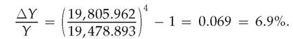
In this case, we say that the annualized quarterly growth rate of GDP in the fourth quarter of 2021 was 0.069 or 6.9%. Note that we can discuss growth rates in decimal terms (0.069) or in growth rates (6.9%), where we can convert a decimal to a percent by multiplying by 100.
If you have annual data, then you would use the same general format as in Eq. (2.12), but you would not raise the ratio of the levels of GDP in Eq. (2.12) to the fourth power because the levels of GDP are for the whole year and so are already annualized. (If you had monthly data, you would raise the ratio in Eq. (2.12) to the 12th power because there are 12 months in a year.) For example, when the GDP growth rate for 2021Q4 of 6.9% was released, the government also released data for the year as a whole. The ratio of real GDP for 2021 to real GDP for 2020 was 1.057, so the growth rate for the year was 0.057 or 5.7%. Thus the fourth quarter growth rate (6.9%) was slightly higher than the growth rate for the year as a whole (5.7%), and the convention of annualizing the growth rate allows a direct comparison.
The convention in the United States is to annualize growth rates of quarterly data.
So, when you read in the news that the growth rate of real GDP was 6.9% in the fourth quarter of 2021, you need to realize that it is an annualized growth rate. However, in many other countries, the government statistical agencies do not follow the same convention. So, if the same numbers were reported in Europe, for example, the GDP growth rate would be reported as 0.017 or 1.7%. The number they report is not annualized, so in Eq. (2.12), the government agency did not raise the ratio to the fourth power.A second convention for U.S. data is that the government statistical agencies report data that are seasonally adjusted, that is, the data are modified to account for normal seasonal variation. The statistical agencies do this to make it easier for users to compare data over the course of a year. For example, many people take long vacations during the summer, so real GDP is lower in the summer months. Many firms gear up production for holiday shopping in November and December, so real GDP in the fall is higher. Some activities such as construction are curtailed in the cold winter months, so real GDP in January and February is lower. Because these seasonal variations are fairly predictable, the statistical agencies seasonally adjust the data to pull out the predictable part of real GDP fluctuations that arise because of these seasonal effects. Similar seasonal adjustment is the norm in other countries, too, but sometimes a country does not seasonally adjust the data because doing so requires a long history so that the statistical agency can accurately detect the seasonal pattern in the data and remove it.
Both the annualization of the data and seasonal adjustment of it are often described by saying the data are "SAAR," which means "seasonally adjusted at an annual rate." So, the next time you hear about a government data report, pay attention to see if it is SAAR, SA and not AR, AR and not SA, or neither.
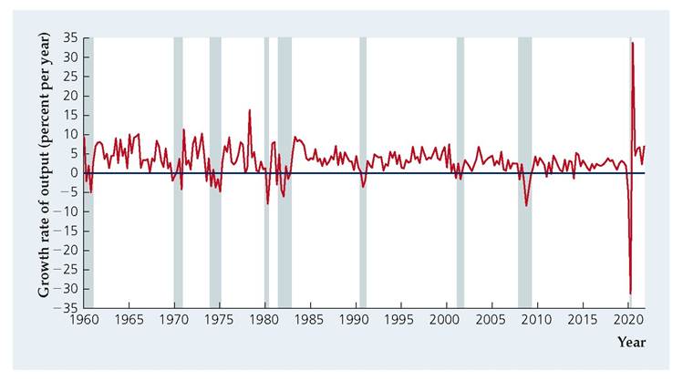
Growth rates of real GDP vary considerably over time.
When the economy enters a recession, the annualized quarterly real GDP growth rate is usually negative. Coming out of a recession, real GDP growth is often very high. To see this, Figure 2.3 shows the SAAR growth rate of real GDP for the United States from 1960Q1 to 2021Q4. Note that the annualized quarterly growth rate is quite volatile. It is easy to pick out periods of recession (shown by green shaded bars), when real GDP growth is often negative.Price Indexes
We have seen how to calculate the portion of the change in nominal GDP owing to a change in physical quantities. Now we turn our attention to the change in prices by using price indexes. A price index is a measure of the average level of prices for some specified set of goods and services, relative to the prices in a specified base year. For example, the GDP deflator is a price index that measures the overall level of prices of goods and services included in GDP, and is defined by the formula 
FIGURE 2.3
The annualized quarterly growth rate of U.S. real GDP, 1960Q1-2021Q4
The quarterly growth rate of U.S. real GDP is annualized by convention to make comparisons between quarterly and annual data easier. The annualized quarterly growth rate is highly volatile and is frequently negative during recessions (shown by green shaded bars).
Source: Bureau of Economic Analysis, National Income and Product Accounts, downloaded from FRED database fred.stlouisfed.org/series/GDPC1.
The GDP deflator (divided by 100) is the amount by which nominal GDP must be divided, or "deflated," to obtain real GDP. In our example, we have already computed nominal GDP and real GDP, so we can now calculate the GDP deflator by rewriting the preceding formula as
GDP deflator = 100 ? nominal GDP/real GDP.
In year 1 (the base year in our example), nominal GDP and real GDP are equal, so the GDP deflator equals 100. This result is an example of the general principle that the GDP deflator always equals 100 in the base year. In year 2, nominal GDP is $66,000 (see Table 2.3) and real GDP is $62,000 (see Table 2.4), so the GDP deflator in year 2 is 100 ? $66,000/$62,000 = 106.5, which is 6.5% higher than the value of the GDP deflator in year 1. Thus the overall level of prices, as measured by the GDP deflator, is 6.5% higher in year 2 than in year 1.
The measurement of real GDP and the GDP deflator depends on the choice of a base year. "In Touch with Data and Research: The Computer Revolution and Chain-Weighted GDP" demonstrates that the choice of a base year can have important effects on the calculated growth of real output, which in turn affects the calculated change in the price level.
In Touch with Data and Research
The Computer Revolution and Chain-Weighted GDP
The widespread use of computers has revolutionized business, education, and leisure throughout much of the developed world. The fraction of the real spending in the United States devoted to computers began to take off in the mid-1980s and continued into the 2000s, while prices of computers fell steadily throughout that period. The sharp increase in the real quantity of computers and the sharp decline in computer prices highlight the problem of choosing a base year in calculating the growth of real GDP.
We can use the example in Tables 2.3 and 2.4, which includes a large increase in the quantity of computers coupled with a sharp decrease in computer prices, to illustrate the problem. We have shown that, when we treat year 1 as the base year, real output increases by 34.8% from year 1 to year 2. However, as we will see in this box using Table 2.4, we get a substantially different measure of real output growth if we treat year 2 as the base year. Treating year 2 as the base year means that we use the prices of year 2 to value output. Specifically, each computer is valued at $600 and each bicycle is valued at $240. Thus the real value of the 5 computers and 200 bicycles produced in year 1 is $51,000. If we continue to treat year 2 as the base year, the real value of output in year 2 is the same as the nominal value of output, which we have already calculated to be $66,000. Thus, by treating year 2 as the base year, we see real output grow from $51,000 in year 1 to $66,000 in year 2, an increase of 29.4%.
Let's summarize our calculations so far. Using year 1 as the base year, the calculated growth of output is 34.8%, but using year 2 as the base year, the calculated growth of output is only 29.4%. Why does this difference arise? In this example, the quantity of computers grows by 100% (from 5 to 10) and the quantity of bicycles grows by 25% (from 200 to 250) from year 1 to year 2. The computed growth of overall output—34.8% using year 1 as the base year or 29.4% using year 2 as the base year—is between the growth rates of the two individual goods. The overall growth rate is a sort of weighted average of the growth rates of the individual goods. When year 1 is the base year, we use year 1 prices to value output, and in year 1 computers are much more expensive than bicycles. Thus the growth of overall output is closer to the very high growth rate of computers than when the growth rate is computed using year 2 as the base year.
Which base year is the "right" one to use? There is no clear reason to prefer one over the other. To deal with this problem, in 1996 the Bureau of Economic Analysis introduced chain-weighted indexes to measure real GDP. Chain-weighted real GDP represents a mathematical compromise between using year 1 and using year 2 as the base year. The growth rate of real GDP computed using chain-weighted real GDP is a sort of average of the growth rate computed using year 1 as the base year and the growth rate computed using year 2 as the base year. (In this example, the growth rate of real GDP using chain-weighting is 32.1%, but we will not go through the details of that calculation here.)[25]
Before the Bureau of Economic Analysis adopted chain-weighting, it used 1987 as the base year to compute real GDP. As time passed, it became necessary to update the base year so that the prices used to compute real GDP would reflect the true values of various goods being produced. Every time the base year was changed, the Bureau of Economic Analysis had to calculate new historical data for real GDP. Chain-weighting effectively updates the base year automatically. The annual growth rate for a given year is computed using that year and the preceding year as base years. As time goes on, there is no need to recompute historical growth rates of real GDP using new base years. Nevertheless, chain-weighted real GDP has a
peculiar feature. Although the income-expenditure identity, Y = C + I + G + NX, always holds exactly in nominal terms, for technical reasons, this relationship need not hold exactly when GDP and its components are measured in real terms when chain-weighting is used. Because the discrepancy is usually small, we assume in this book that the income-expenditure identity holds in both real and nominal terms.
Chain-weighting was introduced to resolve the problem of choosing a given year as a base year in calculating real GDP. How large a difference does chainweighting make in the face of the rapidly increasing production of computers and plummeting computer prices? Using 1987 as the base year, real GDP in the fourth quarter of 1994 was computed to be growing at a 5.1% annual rate. Using chainweighting, real GDP growth during that quarter was a less impressive 4.0%. The Bureau of Economic Analysis estimates that computers account for about three- fifths of the difference between these two growth rates.[26]
20These figures are from p. 36 of J. Steven Landefeld and Robert P. Parker, “Preview of the Comprehensive Revision of the National Income and Product Accounts: BEA's New Featured Measures of Output and Prices,” Survey of Current Business, July 1995, pp. 31-38.
In Touch with Data and Research
Does CPI Inflation Overstate Increases in the Cost of Living?
In 1995-1996 a government commission, headed by Michael Boskin of Stanford University, prepared a report on the accuracy of official inflation measures. The commission concluded that inflation as measured by the CPI may overstate true increases in the cost of living by as much as 1-2 percentage points per year. In other words, if the official inflation rate is 3% per year, the "true" inflation rate may well be only 1%-2% per year.
Why might increases in the CPI overstate the actual rate at which the cost of living rises? One reason is the difficulty that government statisticians face in trying to measure changes in the quality of goods. For example, if the design of an air conditioner is improved so that it can put out 10% more cold air without an increased use of electricity, then a 10% increase in the price of the air conditioner should not be considered inflation; although paying 10% more, the consumer is also receiving 10% more cooling capacity. However, if government statisticians fail to account for the improved quality of the air conditioner and simply note its 10% increase in price, the price change will be incorrectly interpreted as inflation.
Although measuring the output of an air conditioner isn't difficult, for some products (especially services) quality change is hard to measure. For example, by what percentage does the availability of online bill-paying services improve the quality of banking services? To the extent that the CPI fails to account for quality improvements in the goods and services people use, inflation will be overstated. This overstatement is called the quality adjustment bias.
Another problem with CPI inflation as a measure of cost-of-living increases can be illustrated by the following example. Suppose that consumers like chicken and turkey about equally well and in the base year consume equal amounts of each. But then for some reason the price of chicken rises sharply, leading consumers to switch to eating turkey almost exclusively. Because consumers are about equally satisfied with chicken and turkey, this switch doesn't make them significantly worse off; their true cost of living has not been affected much by the rise in the price of chicken. However, the official CPI, which measures the cost of buying the base-year basket of goods and services, will register a significant increase when the price of chicken skyrockets. Thus the rise in the CPI exaggerates the true increase in the cost of living. The problem is that the CPI is based on the assumption that consumers purchase a basket of goods and services that is fixed over time, ignoring the fact that consumers can (and do) substitute cheaper goods or services for more expensive ones. This source of overstatement of the true increase in the cost of living is called the substitution bias.
If official inflation measures do, in fact, overstate true inflation, there are important implications. First, if increases in the cost of living are overstated, then increases in important quantities such as real household income (the purchasing power of a typical household's income) are correspondingly understated. As a result, the bias in the CPI may lead to too gloomy a view of how well the U.S. economy has done over the past few decades. Second, many government payments and taxes are tied, or indexed, to the CPI. Social Security benefits, for example, automatically increase each year by the same percentage as the CPI. If CPI inflation overstates true inflation, then Social Security recipients have been receiving greater benefit increases than necessary to compensate them for increases in the cost of living. If Social Security and other transfer program payments were set to increase at the rate of "true" inflation, rather than at the CPI inflation rate, the Federal government would save billions of dollars each year.
In response to the Boskin Commission's report, the Bureau of Labor Statistics (BLS) made several technical changes in the way it constructs the CPI to reduce substitution bias. These changes have reduced the overstatement of the "true" inflation rate by 0.2 to 0.4 percentage points per year. However, the substitution bias was originally larger than the Boskin Commission's estimate, so the bias in the inflation rate is still 1% per year or perhaps even higher.
Note: For a detailed discussion of biases in the CPI, see David Lebow and Jeremy Rudd, "Measurement Error in the Consumer Price Index: Where Do We Stand?" Journal of Economic Literature, March 2003, pp. 159-201; and Robert J. Gordon, "The Boskin Commission Report: A Retrospective One Decade Later," NBER Working Paper No. 12311, June 2006.
Inflation. An important variable that is measured with price indexes is the inflation rate. The inflation rate equals the percentage rate of increase in the price index per period. Thus, if the GDP deflator rises from 100 in one year to 105 the next, the inflation rate between the two years is (105 — 100)100 = 5/100 = 0.05 = 5% per year. If in the third year the GDP deflator is 112, the inflation rate between the second and third years is (112 — 105)105 = 7/105 = 0.0667 = 6.67% per year. More generally, if Pt is the price level in period t and Pt+1 is the price level in period t + 1, the inflation rate between t and t + 1, or π t+1, is
where , represents the change in the price level from period t
to period t + 1.
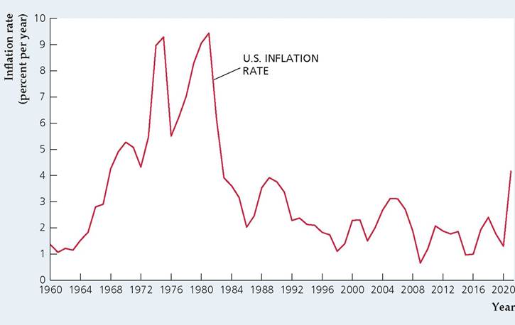
Figure 2.4 shows the U.S. inflation rate for 1960-2021, based on the GDP deflator as the measure of the price level. Inflation rose during the 1960s and 1970s, fell from the early 1980s through the 1990s, and has neither trended upward nor downward since then.
FIGURE 2.4
The inflation rate in the United States, 1960-2021
Here, inflation is measured as the annual percentage change in the GDP deflator. Inflation rose during the 1960s and 1970s, fell from the early 1980s through the 1990s, and has neither trended upward nor downward since then.
Source: Implicit price deflator for GDP, U.S. Bureau of Economic Analysis, downloaded from FRED database, Federal Reserve Bank of St. Louis, fred.stlouisfed.org/series/GDPCTPI.
Application
The Federal Reserve's Preferred Inflation Measures
Our discussion of price indexes describes the GDP deflator and the consumer price index (CPI). But the Federal Reserve (the Fed, for short), in reporting its forecasts of the economy, focuses on a different measure of prices: the personal consumption expenditures (PCE) price index, which is the measure of consumer prices in the national income and product accounts. The Fed announced in November 2007 that it would forecast inflation and other variables four times each year (instead of twice each year as it had done before). It also said that it would forecast both the overall inflation rate in the PCE price index and the core inflation rate of the same index, which excludes food and energy prices.
In the 1990s, the Fed provided forecasts of the inflation rate based on the CPI. But the Boskin Commission's finding (see "In Touch with Data and Research: Does CPI Inflation Overstate Increases in the Cost of Living?") that the CPI measure of inflation substantially overstates increases in the cost of living caused the Fed to move away from focusing on the CPI and to pay more attention to the PCE price index.[27] Because the PCE price index is based on actual household expenditures on various goods and services, it avoids the substitution bias inherent in the CPI.[28] In addition, the Fed suggested that the PCE measure of consumption spending is broader than the CPI, and the PCE measure has the advantage of being revised when better data are available, whereas the CPI is not revised.
Other differences between the CPI and PCE price index include differences in the formulas used to calculate the index, the coverage of different items, and the weights given to different items.[29] The CPI is an index with a given base year whereas the PCE price index is a chain-weighted index, as discussed in "In Touch with Data and Research: The Computer Revolution and Chain-Weighted GDP." The PCE price index covers more types of goods and services, as the CPI is based on the average spending habits of people who live in urban areas, whereas the PCE price index covers all spending on consumer goods in the economy. The weights on different spending categories differ as well; for example, homeownership costs are about 20% of the CPI but only about 11% of the PCE price index.
The Fed used the rate of change of the PCE price index as its main measure of inflation beginning in 2000. Because short-term shocks to food and energy prices can cause sharp, but usually temporary, fluctuations in the inflation rate, the Fed also pays attention to the PCE price index excluding food and energy prices. The inflation rate using this index is called the core PCE inflation rate and the inflation rate that includes inflation in food and energy is called the overall PCE inflation rate. In explaining its use of the core PCE inflation rate, the Fed said that it was a better measure of "underlying inflation trends."[30] Since November 2007 the Fed has provided public forecasts of both core and overall PCE inflation.
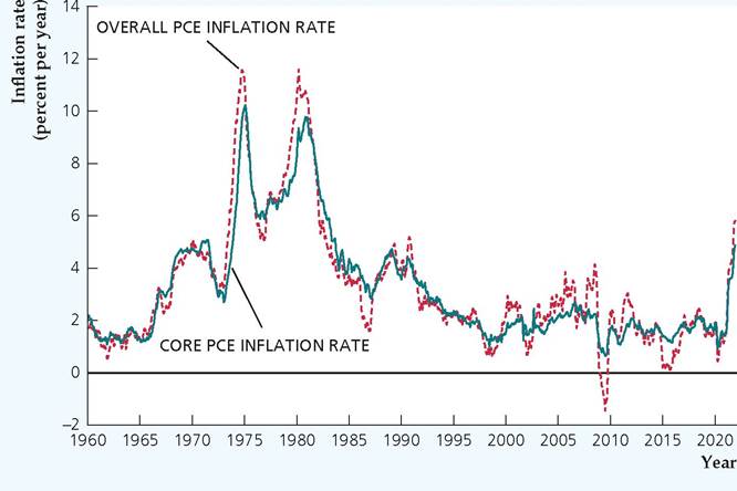
FIGURE 2.5
Overall PCE inflation rate and core PCE inflation rate, January 1960 to December 2021
The overall PCE inflation rate usually differs from the core PCE inflation rate. However, the overall PCE inflation rate tends to revert to the core PCE inflation rate.
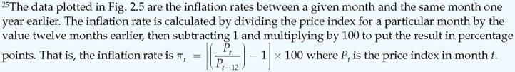
Source: Bureau of Economic Analysis; data downloaded from Federal Reserve Bank of St. Louis FRED database at fred.stlouisfed.org/series/PCEPI and PCEPILFE. Inflation rates are calculated as the percent change in the price index from 12 months earlier.
Figure 2.5 shows how overall PCE inflation differs from core PCE inflation. The figure shows the inflation rates from January 1960 to May 2018.25 You can see in the figure that overall PCE inflation and core PCE inflation differed from each other substantially in many years. Large increases in the price of oil in the mid-1970s and again in the late 1970s caused the overall PCE inflation rate to be above the core PCE inflation rate during these episodes. However, as the relative price of oil declined in the 1980s, the overall PCE inflation rate was less than the core PCE inflation rate from 1982 to 1987. After that, the core PCE inflation rate has not varied as much as the overall PCE inflation rate. Generally, the overall PCE inflation rate tends to revert to the core PCE inflation rate after several years of being above it or below it.
2.5