The Multiplier in the Keynesian Model
In Chapter 11 we defined the multiplier associated with any particular type of spending as the short-run change in total output resulting from a one-unit change in that type of spending.
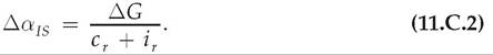
Here we use the analysis in Appendix 9.B to derive the multiplier associated with government purchases G. We proceed in three steps: First, we calculate the effect on αis (the intercept of the IS curve in Eq. 9.B.14) of an increase in G. Then we calculate the effect on the short-run equilibrium value of Y, shown by Eq. (9.B.27), of an increase in αis. Finally, we combine these two effects to calculate the effect on output, Y, of an increase in G.To calculate the effect on αis of an increase in G, we repeat the definition of αis, Eq. (9.B.15):

where c0, i0, cy, cr, ir, and t0 are parameters that determine desired consumption and desired investment (see Appendix 9.B). If G increases by ∆G, then αis increases by ∆G∕(cr + ir), so
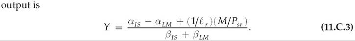
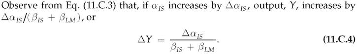
Next, recall from Eq. (9.B.27) that, in the short run when P = Psr, the level of
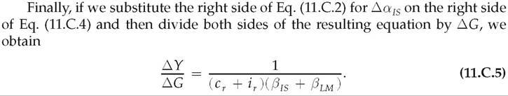
The right side of Eq. (11.C.5) is the increase in short-run equilibrium output, Y, that occurs for each one-unit increase in government purchases, G. In other words, it is the government purchases multiplier.
Similar calculations show that changesin desired consumption or desired investment (as reflected in the terms c 0 and i 0) have the same multiplier as government purchases.
Because , and,
 all are positive, the multiplier is positive. However,
depending on the specific values of those parameters, the multiplier may be greater or less than 1. A case in which the multiplier is likely to be large occurs when the LM curve is horizontal (that is, when the slope of the LM curve, is 0). If the LM curve is horizontal, shifts in the IS curve induced by changes in spending have relatively large effects on output. Recall that Eq. (9.B.16) gives the (negative of the) slope of the IS curve,
 .. Making this substitu
tion and setting the slope of the LM curve,361" class="lazyload" data-src="/files/uch_group77/uch_pgroup317/uch_uch7363/image/image360.jpg">, at 0 yield a simple form of the multiplier:
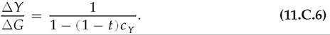
For example, suppose that the marginal propensity to consume, cγ, is 0.8 and that the tax rate, t, is 0.25. Then the multiplier defined in Eq. (11.C.6) is 1∕[ 1 — (0.75)(0.8)] = 1/0.4, or 2.5. If the LM curve is very steep, by contrast—that is, eLM is large—then the multiplier could be quite small, as you can see from Eq. (11.C.5).
More on the topic The Multiplier in the Keynesian Model:
- The Multiplier in the Keynesian Model
- Worked-Out Numerical Exercise for Calculating the Multiplier in a Keynesian Model
- The Samuelson Multiplier Accelerator Model
- 8 The Keynesian Model of Income Determination in a Four Sector Economy: Introduction of the Foreign Sector
- 7 The Keynesian Model of Income Determination in a Three Sector Economy: Introduction of the Government Sector
- The Original Keynesian Models
- Conclusion
- American Keynesianism
- Monetary and Fiscal Policy in the Keynesian Model
- Contents