Transitional Dynamics in the Continuous Time Solow Model
The analysis of transitional dynamics and stability with continuous time yields similar results to those in Section 2.3, but in many ways simpler. To do this in detail, we need to remember the equivalents of the above theorems for differential equations.
The following theorems follow from the results presented in Appendix Chapter B.Theorem 2.4. Consider the following linear differential equation system
(2.34) 
with initial value x (0), where x (t) ∈ Rn for all t, A is an n ? n matrix and b is a n ? 1 column vector. Let x* be the steady state of the system given by Ax* + b = 0. Suppose that all of the eigenvalues of A have negative real parts. Then the steady state of the differential equation
(2.34) x* is globally asymptotically stable, in the sense that starting from any x (0) ∈ Rn, x(t) → x*.
Theorem 2.5. Consider the following nonlinear autonomous differential equation
(2.35) 
with initial value x (0), where be a steady state of this system, i.e.,
G (x*) = 0, and suppose that G is continuously differentiable at x*. Define
and suppose that all of the eigenvalues of A have negative real parts. Then the steady state of the differential equation (2.35) x* is locally asymptotically stable, in the sense that there 59

Once again an immediate corollary is:
Corollary 2.2. Let x (t) ∈ R, then the steady state of the linear difference equation x (t) = ax (t) is globally asymptotically stable (in the sense that x (t) → 0) if a < 0.
Let g : R → R be continuous and differentiable at x* where g (x*) = 0. Then, the steady state of the nonlinear differential equation x (t) = g (x (t)), x*, is locally asymptotically stable if g' (x*) < 0.
Proof. See Exercise 2.8. ?
Finally, with continuous time, we also have another useful theorem:
Theorem 2.6. Let g : R → R be a continuous function and suppose that there exists a unique x* such that g (x*) = 0. Moreover, suppose g (x) < 0 for all x > x* and g (x) > 0 for all x < x*. Then the steady state of the nonlinear differential equation x (t) = g (x (t)), x*, is globally asymptotically stable, i.e., starting with any x (0), x (t) → x*.

Notice that the equivalent of Theorem 2.6 is not true in discrete time, and this will be illustrated in Exercise 2.14.
In view of these results, Proposition 2.5 immediately generalizes:
PROPOSITION 2.9. Suppose that Assumptions 1 and 2 hold, then the basic Solow growth model in continuous time with constant population growth and no technological change is globally asymptotically stable, and starting from any k (0) > 0, k (t) → k*.
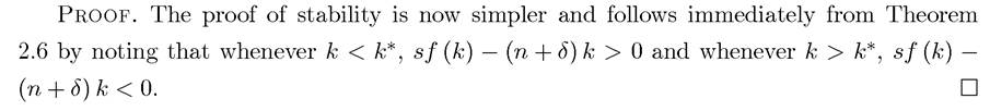
Figure 2.9 shows the analysis of stability diagrammatically. The figure plots the righthand side of (2.32) and makes it clear that whenever ę < ę*, ę > 0 and whenever ę > ę*, ę < 0, so that the capital-effective labor ratio monotonically converges to the steady-state value k*.
Example 2.2. (Dynamics with the Cobb-Douglas Production Function) Let us return to the Cobb-Douglas production function introduced in Example 2.1

60
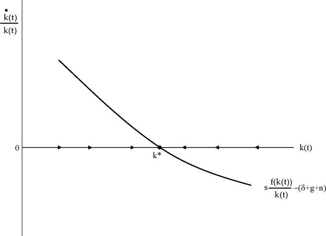
Figure 2.9. Dynamics of the capital-labor ratio in the basic Solow model.
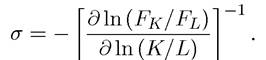
As noted above, the Cobb-Douglas production function is special, mainly because it has an elasticity of substitution between capital and labor equal to 1. Recall that for a homothetic production function F (K,L), the elasticity of substitution is defined by
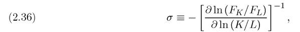
where Fk and /7. denote the marginal products of capital and labor. In addition, F is required to be homothetic, so that Fk/Fl is only a function of K∕L. For the Cobb-Douglas production function Fk/Fl = (α∕ (1 — α)) ∙ (L∕K), thus σ = 1. This feature implies that when the production function is Cobb-Douglas and factor markets are competitive, equilibrium factor shares will be constant irrespective of the capital-labor ratio. In particular:
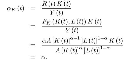
Similarly, the share of labor is The reason for this is that with an elasticity
of substitution equal to 1, as capital increases, its marginal product decreases proportionally, leaving the capital share (the amount of capital times its marginal product) constant.
Recall that with the Cobb-Douglas technology, the per capita production function takes the form f (k) = Akα, so the steady state is given again from (2.33) (with population growth at the rate n) as  or
or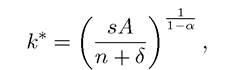
which is a simple and interpretable expression for the steady-state capital-labor ratio. k* is increasing in s and A and decreasing in n and δ (which is naturally consistent with the results in Proposition 2.8). In addition, k* is increasing in α. This is because a higher α implies less diminishing returns to capital, thus a higher capital-labor ratio reduces the average return to capital to the level necessary for steady state as given in equation (2.33).
Transitional dynamics are also straightforward in this case. In particular, we have:
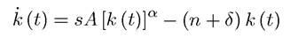
with initial condition k (0). To solve this equation,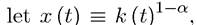 so the equilibrium
law of motion of the capital labor ratio can be written in terms of x (t) as

which is a linear differential equation, with a general solution
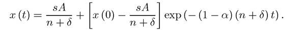
(see, for example, the Appendix Chapter B, or Boyce and DiPrima, 1977, Simon and Bloom, 1994). Expressing this solution in terms of the capital-labor ratio

This solution illustrates that starting from any k (0), the equilibrium k (t) → k* = 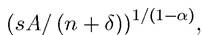 and in fact, the rate of adjustment is related to (1 — α)(n + δ), or more specifically, the gap between k (0) and its steady-state value is closed at the exponential rate (1 — α)(n + δ). This is intuitive: a higher α implies less diminishing returns to capital, which slows down the rate at which the marginal and average product of capital declines as capital accumulates, and this reduces the rate of adjustment to steady state. Similarly, a smaller δ means less replacement of depreciated capital and a smaller n means slower population growth, both of those slowing down the adjustment of capital per worker and thus the rate of transitional dynamics.
EXAMPLE 2.3. (The Constant Elasticity of Substitution Production Function) The previous example introduced the Cobb-Douglas production function, which featured an elasticity of substitution equal to 1.
The Cobb-Douglas production function is a special case of the constant elasticity of substitution (CES) production function, first introduced by Arrow, Chenery, Minhas and Solow (1961). This production function imposes a constant elasticity, σ, not necessarily equal to 1. To write this function, consider a vector-valued index of technology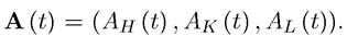 Then the CES production function can be written
 as
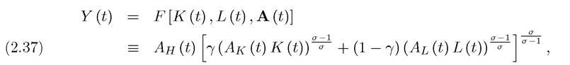
where Ah (t) > 0, Ak (t) > 0 and Al (t) > 0 are three different types of technological change which will be discussed further in Section 2.6; γ ∈ (0,1) is a distribution parameter, which determines how important labor and capital services are in determining the production of the final good and σ ∈ [0, ∞] is the elasticity of substitution. To verify that σ is indeed the constant elasticity of substitution, let us use (2.36). In particular, it is easy to verify that the ratio of the marginal product of capital to the marginal productive labor, Fk/Fl, is given by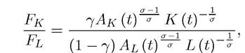
thus, we indeed have that
The CES production function is particularly useful because it is more general and flexible than the Cobb-Douglas form while still being tractable. As we take the limit σ → 1, the CES production function (2.37) converges to the Cobb-Douglas function Y (t) =  As
As the CES production function
becomes linear, i.e.

Finally, as σ → 0, the CES production function converges to the Leontief production function with no substitution between factors,


reduction in capital or labor will have no effect on output or factor prices.
Exercise 2.16 illustrates a number of the properties of the CES production function, while Exercise 2.17 63provides an alternative derivation of this production function along the lines of the original article by Arrow, Chenery, Minhas and Solow (1961).
2.5.1. A First Look at Sustained Growth. Can the Solow model generate sustained growth without technological progress? The answer is yes, but only if we relax some of the assumptions we have imposed so far.
The Cobb-Douglas example above already showed that when α is close to 1, adjustment of the capital-labor ratio back to its steady-state level can be very slow. A very slow adjustment towards a steady-state has the flavor of “sustained growth” rather than the economy settling down to a stationary point quickly.
In fact, the simplest model of sustained growth essentially takes α = 1 in terms of the Cobb-Douglas production function above. To do this, let us relax Assumptions 1 and 2 (which do not allow α = 1), and suppose that

where A > 0 is a constant. This is the so-called “AK” model, and in its simplest form output does not even depend on labor. The results we would like to highlight apply with more general constant returns to scale production functions, for example,

but it is simpler to illustrate the main insights with (2.38), leaving the analysis of the richer production function (2.39) to Exercise 2.15.
Let us continue to assume that population grows at a constant rate n as before (cfr. equation (2.31)). Then, combining this with the production function (2.38), the fundamental law of motion of the capital stock becomes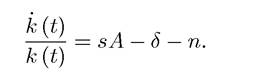
Therefore, if the parameters of the economy satisfy the inequality sA — δ — n> 0, there will be sustained growth in the capital-labor ratio. From (2.38), this implies that there will be sustained growth in output per capita as well. This immediately establishes the following proposition:
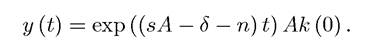
Proposition 2.10. Consider the Solow growth model with the production function (2.38) and suppose that sA — δ — n > 0. Then in equilibrium, there is sustained growth of output per capita at the rate sA — δ — n. In particular, starting with a capital-labor ratio k (0) > 0, the economy has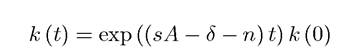
and
64
This proposition not only establishes the possibility of endogenous growth, but also shows that in this simplest form, there are no transitional dynamics. The economy always grows at a constant rate sA — δ — n, irrespective of what level of capital-labor ratio it starts from. Figure 2.10 shows this equilibrium diagrammatically.
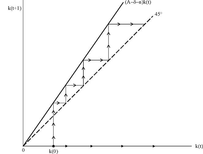
Figure 2.10. Sustained growth with the linear AK technology with sA — δ — n > 0.
Does the AK model provide an appealing approach to explain sustained growth? While its simplicity is a plus, the model has a number of unattractive features. First, it is a somewhat knife-edge case, which does not satisfy Assumptions 1 and 2; in particular, it requires the production function to be ultimately linear in the capital stock. Second and relatedly, this feature implies that as time goes by the share of national income accruing to capital will increase towards 1. We will see in the next section that this does not seem to be borne out by the data. Finally and most importantly, we will see in the rest of the book that technological progress seems to be a major (perhaps the most major) factor in understanding the process of economic growth. A model of sustained growth without technological progress fails to capture this essential aspect of economic growth. Motivated by these considerations, we next turn to the task of introducing technological progress into the baseline Solow growth model.
2.6.
More on the topic Transitional Dynamics in the Continuous Time Solow Model:
- Transitional Dynamics in the Continuous Time Solow Model
- Acemoglu Daron. Introduction to Modern Economic Growth: Parts 1-4. Department of Economics, Massachusetts Institute of Technology,2008. — 604 p., 2008
- Contents
- Table of contents
- Transitional Dynamics in the Discrete Time Solow Model
- Transitional Dynamics in the DiscreteTime Solow Model
- Acemoglu D.. Introduction to Modern Economic Growth. Princeton University Press,2008. — 1248 p., 2008
- References and Literature
- Solow Model and Regression Analyses
- Solow Model with Technological Progress