Money and monetary policy
This chapter looks at the nature of money and the functions any money commodity must perform, before considering its importance from both monetarist and Keynesian perspectives. Before the money stock can be monitored and its effect on the economy considered, it must be measured.
We therefore look at current definitions of the money stock, distinguishing between ‘narrow’ money and ‘broad’ money. We review the rules versus discretion debate and consider the importance of credibility and transparency. The development of monetary policy and the emergence of targets is considered with an emphasis on inflation targeting.The increasing emphasis of governments and central banks on using monetary policies to avoid deflation is examined. The problems associated with the deflationary tendencies in the global economy since the 2007 sub-prime market collapse are reviewed, together with the monetary techniques now being adopted to tackle those problems! Particular attention is paid to the use of ‘quantitative easing’ and the impacts this approach is having on the real economies of the UK, US and Japan amongst others.
I The nature of money
We are all familiar with money. We use it almost every day of our lives, we recognize it when we see it, and most of us are all too aware that we don’t have enough of it! Despite this, the effect of changes in the money supply on macroeconomic variables such as the rate of inflation, the rate of unemployment and the level of output are matters of deep controversy. One reason for this is that there is no completely watertight physical or legal definition of money. Instead, economists adopt a behavioural approach to the definition of money. This approach highlights the confidence element of money and emphasizes the importance of its acceptability. At the most basic level, money can be thought of as anything generally acceptable to others as a means of payment.
History is littered with examples of commodities that have functioned as money at different times and in different places. The word ‘pecuniary’ is derived from the Latin for cattle and ‘salary’ is derived from the Latin for salt, indicating that both these commodities have functioned as money in the past. Other commodities such as stones, shells, beads and metals have also functioned as money.In the UK, notes, coins, cheques and credit cards are used as means of payment to promote the exchange of goods and services and to settle debts, but cheques and credit cards are not strictly regarded as part of the money supply. Rather it is the underlying bank deposit of the cheque or credit card which is part of the money supply. Since cheques are simply an instruction to a bank to transfer ownership of a bank deposit, a cheque drawn against a non-existent bank deposit will be dishonoured by a bank and the debt will remain, as will also be the case if an attempt is made to settle a transaction by using an invalid credit card. Therefore a general definition of money in the UK today is notes, coins and bank and building society deposits.
In practice, for any asset to be considered as money it must perform certain functions and we turn now to a brief discussion of these.
I Functions of money
Unit of account
One of the most important functions of money is to serve as a numeraire, or unit of account. Distance is measured in metres, weight in kilograms and so on. In the same way, when we measure the relative value in exchange of a house, a car or a haircut, our measuring rod is money. Money is therefore a common denominator against which value in exchange can be expressed. We then know that a litre of petrol is less valuable than a litre of whisky because we are able to express relative values in money terms. In the UK the basic unit of account is the pound sterling and all values in the UK are expressed in pounds sterling or fractions of a pound sterling.
The existence of a unit of account facilitates rational decision-taking by consumers and producers.
To understand the importance of this, consider a barter economy, i.e. an economy in which there is no unit of account. As an initial simplification, assume that only four consumer goods are offered for sale in this economy. To make decisions about how much of each good to acquire, consumers would need to consider the value of each good in relation to the value of all other goods. Figure 20.1(a) shows that consumers would need to express the value of good A in terms of goods B, C and D. Similarly, the value of good B would need to be expressed in terms of goods A, C and D, and so on. Without money, each good or service offered for sale would require an exchange value (or ratio) expressed in terms of each of the other goods and services offered for sale; six exchange ratios in all would be required. Figure 20.1(b) shows that when a unit of account does exist, the number of exchange ratios is reduced (here to only three) because the value of each good can be expressed in terms of the money commodity.This is important because the number of exchange ratios increases rapidly as the number of goods and services offered for sale increases. In fact, we can calculate the number of exchange ratios that would exist in a barter economy if we substitute into the formula:
Rb = 1N(N - 1)
where Rb = the number of exchange ratios in a barter economy;
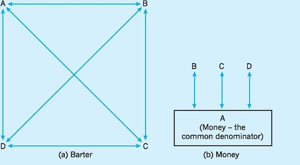
Fig. 20.1 (a) In a non-money economy producing four goods, six exchange ratios are required. (b) In a money economy producing four goods where one of the goods is money, only three exchange ratios are required.
N = the number of goods and services traded in the barter economy.
For example, in an economy where 1,000 goods and services are traded (quite a modest number compared with the number of goods and services actually traded in a modern economy such as the UK), the number of exchange ratios that would exist is 499,500! Imagine trying to make rational decisions about what and how much to produce when it is first necessary to compare such a large number of exchange ratios.
Contrast this situation with the number of exchange ratios that exist in a money economy and you immediately see one of the main advantages of money. In this case the number of exchange ratios is simply:
Km = N - 1
where Km = the number of exchange ratios in a money economy;
N = the n umber of goods and services traded in the money economy.
Again, if 1,000 goods and services are traded, the number of exchange ratios is now only 999 for the money economy. Since each of these exchange ratios is expressed in the same unit of account, comparisons between relative goods and services as regards exchange value is very easy, taking the form of relative prices in a money economy. The fact that it is easy to compare relative prices makes it possible for consumers and producers to estimate the opportunity cost of any production or consumption decision. Economic theory tells us that in these circumstances resources are likely to be allocated much more efficiently than would otherwise be the case.
Medium of exchange
In this sense, money is an interface between buyers and sellers which enables them to trade without the existence of a ‘double coincidence of wants’. With a barter system those who trade must seek out others who have what they require and in turn require what they have. In functioning as a medium of exchange, money greatly improves the efficiency of the economic system and vastly increases the scope for specialization, thereby allowing firms to achieve economies of scale. So important is the role of money in the process of exchange that it would be impossible for all but the most primitive societies to function in the absence of money.
The restrictions on specialization and exchange that would characterize a barter economy are easy to illustrate. Consider a producer of wheat who requires cloth. First the wheat producer must find someone who requires wheat and who is simultaneously able to offer cloth in exchange. Having established such a double coincidence of wants, it is then necessary to agree a mutually acceptable rate of exchange for wheat in terms of cloth.
In such cases, the time and effort devoted to exchange might well exceed that devoted to production and there would be a tendency towards self-sufficiency.Compare this with a money economy where the process of trade simply involves the exchange of money in return for the receipt of goods or services. Money clearly makes specialization and trade viable, but it also makes possible the vast economies of scale so characteristic of modern production. Remember, mass production is impossible without the existence of a mass market, and the existence of a common medium of exchange within an economy satisfies one of the conditions necessary for the existence of such a mass market. Without money it would be impossible for countries to support their current populations, far less for them to enjoy their current standard of living.
Store of value
The store of value function of money is closely bound up with its medium of exchange function. As a store of value, money permits a time-lag to exist between the sale of one thing and the purchase of something else. When goods and services are sold they are purchased with money which is then held by the sellers of goods and services until they themselves make purchases. In this sense, money is an asset used for storing the value of sales until this value is required to make purchases. Most people receive payment for their labour at discrete intervals, usually a week or month, which do not coincide with the continuous flow of expenditures made over the same period. Money is therefore a convenient form in which to store purchasing power.
Money is not unique as a store of value and there are many forms in which wealth can be held, ranging from financial assets such as government bonds, to physical assets such as antiques. As a means of storing wealth these assets have advantages over money. For example, holders of government bonds receive interest income while holders of antiques usually experience a capital gain. Money, on the other hand, has the advantage of being immediately acceptable in exchange for goods and services.
Economists use the term liquidity to describe assets which can easily and inexpensively be converted into money. Money is therefore the most liquid of all assets.The liquidity which money possesses gives it a ‘convenience value’ over other assets, but whether it is an effective store of value depends on the behaviour of the price level. The nominal value of money is fixed by law, but during periods of inflation, when prices rise, the real value of money falls. Clearly as inflation rises, money performs its store of value function less and less effectively. Indeed, inflation can be thought of as a tax on money holdings and the tax rate is equal to the rate of inflation. For example, between 31st July 2009 and 31st July 2010 the Consumer Price Index (CPI) in the UK increased from 110.9 to 114.3. This implied that the purchasing power of £1.00 on 31 July 2009 had a purchasing power of £0.97 on 31 July 2010, as the following calculation shows.
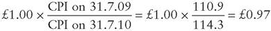
Between 31 July 2009 and 31 July 2010, the real value of money had fallen by 3%.
The store of value function of money and the medium of exchange function are closely bound together. In periods of hyperinflation, money ceases to function both as an effective store of value and as an effective medium of exchange. Indeed, those hyperinflations that have been documented are characterized by economic agents spending money balances as quickly as possible before they become worthless. A classic example of this occurred during the French Revolution of 1789 when assignants, the paper currency of the time, were issued in such quantity that their value declined so quickly that the peasants used them for the most ignominious purpose to which paper can ever be put. The German experience with hyperinflation in the inter-war period provides another classic example of money becoming ineffective as both a store of value and a medium of exchange. In extreme cases such as this, the value of money falls so quickly that it becomes increasingly difficult to make production and investment decisions. The result is that economic activity declines and economic agents resort to barter and exchange goods and services directly. The growth of the ‘barter economy’ during the hyperinflation in Zimbabwe in recent years is a case in point.
A standard for deferred payments
Economists sometimes identify a fourth function of money: that it provides a standard for deferred payments. In this sense, money provides a means of agreeing payments to be made at some future date, at the time when contracts are signed. Arguably, this is simply a particular aspect of its unit of account function.
Near money
Commodities which fulfil only some of the functions of money cannot be classed as money. Credit cards and luncheon vouchers, for instance, can sometimes be used as a medium of exchange for transactions, but they are not money because they cannot always be used and neither do they fulfil the other functions of money. Paper assets such as government securities serve as a store of value, but they cannot be used as a medium of exchange. However, liquid assets, i.e. those which can easily be converted into money without loss of value, form a potential addition to the money stock, and are often referred to as ‘near money’. Assets normally classed as ‘liquid’ include time deposits, treasury and commercial bills, and certificates of deposit (Fig. 20.2). Other assets become more liquid the nearer they are to their maturity date. Many of the assets shown in Fig. 20.2 are considered in more detail later in this chapter and in Chapter 21.
Electronic money
The creation and use of electronic money, though still in its infancy, is likely to increase rapidly over the next few years. The possible implications of this are profound and far-reaching. So what is electronic money? Electronic money is a payment instrument whereby monetary value is stored electronically on some device in the possession of the customer. The European Central Bank defines electronic money as ‘an electronic store of monetary value on a technical device that may be widely used for making payments to undertakings other than the issuer without necessarily involving bank accounts in the transaction, but acting as a prepaid bearer instrument’.
The most obvious device for storing money is a computer chip embedded in a smart card and, for purposes of simplicity, our discussion here is restricted to this. The amount stored on the chip is increased or decreased every time it is used in some financial transaction or whenever funds are loaded onto, or unloaded from, the card. In this way, electronic money stored on a card can be thought of as being similar to cash stored in a wallet. The amount of money in the wallet goes up or down according to whether purchases or sales take place and additional balances can be loaded into the wallet or unloaded from it. This is entirely different from a credit card which simply gives its owner an immediate overdraft. E-money more closely resembles cash than credit card transactions, and Fig. 20.3 shows the clearing and settlement of cash and E-money.
E-money is convenient and settlement is almost immediate. It is possible for E-money users to transfer balances onto their stored value cards from home and terminals that accept E-money transfer funds stored on a chip, into a bank account in settlement of transactions, almost invariably without delay. Another advantage of E-money is that it eliminates the necessity of carrying coins, which most people find inconvenient since they inevitably pile up in pockets and purses! The problems with E-money include consumer resistance because of loss of anonymity when making transactions and consumer concerns over security and the possibility of counterfeiting. These
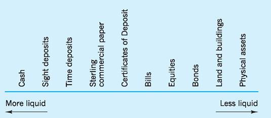
Fig. 20.2 Liquidity spectrum.
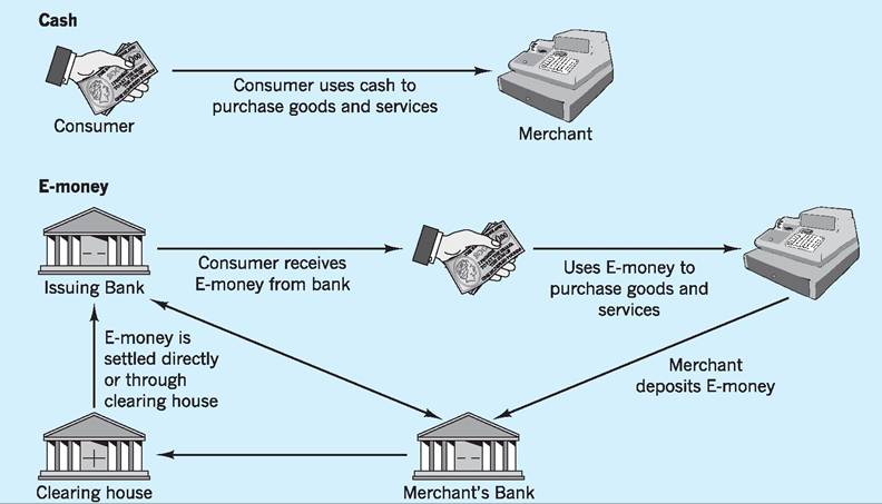
Fig. 20.3 Clearing and settlement of cash and E-money. Source: Rossell (1997), p. 6.
problems are technical and can probably be overcome relatively easily. For example, some institutions provide anonymity by offering E-money which, once it has been downloaded onto the card and balances are transferred from the individual’s to the institution’s account, cannot be ‘matched’ to the account from which it originated. Security and counterfeiting risks can probably be minimized by the development of sophisticated encryption techniques. When these are available and the public has trust in them, the use of E-money is likely to rise substantially.
The importance of money
Economists are in no doubt that ‘money matters’, but there is considerable disagreement as to how changes in the money stock influence macroeconomic variables (the so-called transmission mechanism) and as to the magnitude of its influence on these variables. Monetarists argue that although changes in the rate or growth of the money supply may influence ‘real’ variables such as output and employment in the short run, in the long run they affect only nominal (or money) variables such as the rate of inflation, the rate of interest and the rate of exchange. The neoclassical view is an extension of monetarist thinking and agrees that changes in the rate of growth of the money supply affect only nominal variables, but contends that this is the case in both the long run and the short run. Keynesians, on the other hand, argue that as well as affecting nominal variables, changes in the rate of growth of the money supply also affect real variables such as the level of output and employment in both the short run and the long run.
It is natural that we should focus on the differences between Keynesians and monetarists, but it would be a mistake to think that there are no similarities! Both groups agree that in the short run an increase in money supply will affect both real and nominal variables. They also agree that nominal variables will be affected in the long run, but they disagree over the nature of the transmission mechanism and over the influence of changes in money supply on the real economy in the long run. Keynes held the view that higher inflation was an acceptable price to pay for higher output and employment. Although he never specified what rate of inflation would be ‘acceptable’, it is likely that he had in mind some relatively low rate such as the 2% per annum currently targeted by the Bank of England. Monetarists, on the other hand, argue that any changes in output and employment that occur as a result of higher money growth will be only transitory, i.e. in the long-run real variables will revert back to their equilibrium rates and higher money supply will affect only nominal variables.
The quantity theory of money
The relationship between money on the one hand and nominal income (final output ? the average price of that output) on the other is formally recognized in the equation of exchange. The income version of this states that:
M ? Vy = P ? Y
In other words, over any given time period, the amount of money in circulation (M) times the income velocity of circulation (Vy) (i.e. the average number of times the money supply is spent on final output) must be identical to the average price of final output (P) times the volume of final output produced (Y).
Note that the income velocity of circulation (Vy) is a measure of the speed at which money is spent on final output and is determined by several factors. One important factor is the frequency with which payments are made. For example, if wages are paid monthly and all other things are equal, money balances will, on average, be higher than if wages are paid weekly. This implies a lower income velocity of circulation.
There is nothing controversial in the equation of exchange. It is simply an identity and must be true by definition. It simply tells us that the value of spending on final output in one period (MVy) equals the value of output purchased in the same period (PY). However, if we assume that Vy and Y are constant, then we have a relationship between M and P.
The quantity theory of money specifies the nature of this relationship and states that the relationship is causal from money to prices. In other words, an increase in the money supply will cause an increase in the average price level. Furthermore, causation is one way, that is, the average price level cannot change unless there has been a prior change in the money supply. We shall see below that this strict interpretation of the quantity theory of money remains controversial.
The monetarist view of money
The quantity theory of money is the basis of all monetarist thinking. In short, monetarism is a set of beliefs about the ways in which changes in money growth (the rate of growth of the money supply) affect other macroeconomic variables. Monetarists argue that, in the short run, the effect of changes in money growth is ambiguous, affecting both real variables (output, employment, real wages, etc.) and nominal variables (the rate of inflation, the rate of interest, the rate of exchange, etc.), though in imprecise and largely unpredictable ways. However, in the long run the effect of changes in money growth is unambiguous, affecting only nominal variables. It is for this reason that monetarists focus on long-run relationships.
Monetarist beliefs are based on empirical relationships which they claim show a highly significant correlation between money growth and nominal national income. However, since they believe that real national income (output) is not affected by changes in money growth in the long run, the implication is that increased money growth leads to higher nominal income through inflation. In other words, increases in money growth lead, in the long run, to an increase in the rate of inflation.
The demand for money
All monetarists accept the quantity theory of money, but the emergence of monetarism as an economic doctrine focuses on the demand for money. Monetarists argue that the demand for money is determined by the same general factors which influence the demand for other goods and services and focus particularly on the level of income, the price level and the expected rate of inflation. It is claimed that the relationship between these variables and the demand for money is stable over time. This is an extremely important claim because such stability could not exist unless the velocity of circulation was also constant. In other words, if it can be shown that the demand for money is stable, then the income velocity of circulation (Vy) is also stable.1
For simplicity, the monetarist view implies that the demand for money is a stable function of nominal national income. The reasoning underlying this view is that in the long run the actual rate of inflation and the expected rate of inflation coincide. The main determinants of changes in the demand for money are
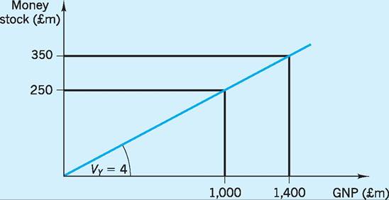
Fig. 20.4 When velocity of circulation is constant, a change in the money supply leads to a proportional change in nominal GDP.
therefore changes in the actual rate of inflation, that is, the rate of change of the price level, and changes in real income, that is, changes in nominal GNP divided by the price level. Monetarists therefore argue that when there is increased money growth, this will lead to changes in nominal GNP which will restore equilibrium between the demand for money and the supply of money.
To understand this more fully, the equation of exchange (MVγ = PY) can be written in the form M = kPY where k = 1/VY. In equilibrium, the demand for money equals the supply of money and so we can write:
Ms = Md = kPY
Note that k is the proportion of nominal income (PY) that the population demand as money. Beginning with equilibrium between demand for money and supply of money, if the supply of money increases there will be disequilibrium between demand for money and supply of money. How is equilibrium restored? If, as the monetarists assume, Vy is constant, then k must also be constant and equilibrium can only be restored by a rise in nominal income (PY). If Vy is not stable, then k will not be stable. In this case, equilibrium following an increase in the money supply might be partially or totally restored by a change in the proportion of national income held as money. In other words, equilibrium is restored by a change in the demand for money that is not proportionately related to a change in nominal income.
Figure 20.4 is used as a basis for explanation. If the demand for money is constant at 25% of GNP, that is k = 4, and the initial level of GNP is £1,000m then, assuming that demand for money and supply of money are in equilibrium, the quantity of money supplied and demanded is £250m. If the money supply now increases, nominal GNP will increase and, since k is assumed to be constant, demand for money will also increase. For example, if the money supply increases by £100m, equilibrium will be restored when demand for money increases by £100m and, with k constant at 4, this implies that GNP increases to £1,400m.
The transmission mechanism
An important question to answer is why nominal GNP increases following an increase in money growth. In fact, the route by which the effect of a change in the money supply is transmitted to the economy is referred to as the transmission mechanism. The monetarists argue that an increase in the money supply will leave people holding excess money balances at the existing level of GNP. Consequently, spending on a whole range of goods and services will increase as economic agents (individuals and organizations) divest themselves of unwanted holdings of money. (This contrasts with liquidity preference theory which implies that it will be spent on securities - see the following section.) As aggregated demand increases, output and prices will rise until people are persuaded to hold an amount of money equivalent to the increased money supply in order to finance the increased value of their transactions. In other words, nominal GNP goes on rising until the increase in the supply of money is matched by an increase in the transactions demand for money, so that supply an demand for money are brought back into equilibrium.
However, this simple approach is ambiguous because an increase in nominal GNP can consist entirely of an increase in real income with prices unchanged, or entirely of an increase in prices with real income unchanged, or some combination of both. The monetarists claim that in the short run, the increase in nominal GNP will consist of an increase in both real income (output) and prices. However, in the long run they argue that there is an equilibrium ‘natural rate of output’ which is determined by institutional factors such as the capital stock, mobility of labour, the rate of social security payments, whether a minimum wage exists and so on (see Chapter 23). Such factors are not influenced by changes in money growth. Whilst it is possible that changes in money growth will bring about changes in real income in the short run, such changes will be only transitory since in the long run real income will return to the level that would have existed before the increase in money growth. Hence, an increase in money growth above the rate of growth of real income will, in the long run, simply lead to higher prices.
Short-run and long-run adjustment to a monetary shock
But why should output increase in the short run following an increase in money growth, and return to the ‘natural rate’ in the long run? In fact, an increase in money growth encourages increased spending as economic agents attempt to divest themselves of excess money balances at the existing price level. The inevitable consequence is rising prices. This implies a fall in real wages and an increase in the real profits of firms, providing the incentive to increase production. However, over time, rising prices are followed by rising nominal wages. The mechanism is now reversed. When the real wage is restored, real profits revert to their original level and the incentive to increase production (higher real profits) disappears. As a consequence, firms cut back on production and output reverts to the ‘natural rate’. In terms of the quantity theory, the implication is that both velocity and output are constant in the long run and that an increase in money growth merely causes an increase in prices.
Criticisms of the quantity theory
It is important to note that monetarism changes the relationship between M and P (given Vy and Y) from that of an identity to that of a causal relationship. Although monetarism provides a theoretical rationale for doing this, a number of criticisms can be made of the view that a change in M will automatically lead, in the long run, to a proportionate change in P.
The first and perhaps most damaging criticism relates to assumptions about the behaviour of the velocity of circulation. The velocity has always fluctuated in the short run, sometimes in response to sudden changes in money growth. In the longer run, however, monetarists argue that velocity is relatively stable. Indeed Fig. 20.5 provides rather ambiguous evidence as to the stability of the velocity of the broad money aggregate M4 (see p. 406 below) and more serious statistical analysis is necessary to test for stability. Such testing is beyond the scope of this chapter, but it is fraught with difficulty as the following section explains.
Figure 20.5 does not provide conclusive evidence so that the debate about whether the velocity of circulation (Vy) can be regarded as stable in the long run is far from over. In fact, there is widespread agreement that velocity is unstable in the short run, though economists cannot agree about its behaviour in the long run. A considerable amount of research has been undertaken to test the stability of the demand for money function (remember, if demand for money is stable, velocity is stable), with mixed results. One reason for this is that there is no accepted definition of what constitutes the short run. Indeed, many economists who accept the predictions of the quantity theory allege that the length of the short run is variable and subject to unspecified changes in duration. This, of course, makes empirical testing of the quantity theory extremely difficult. It is therefore very difficult to identify the short-run influences on the demand for money and to assess their effects. There are also problems with the way in which the money supply is measured and hence with the way in which velocity is calculated.2 In this respect, some economists have argued that no simple monetary aggregate sum measure of money such as M4 is a particularly
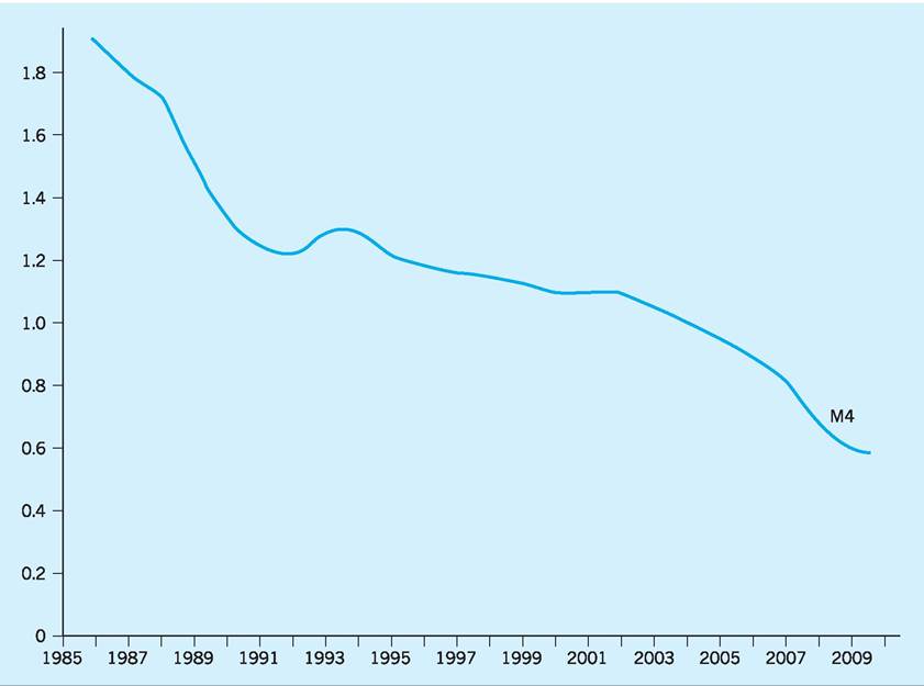
Fig. 20.5 Velocity of the money aggregate M4. Source: ONS Financial Statistics (various).
useful measure of money and that the Divisia (see p. 406) is superior.
A further problem with the monetarist explanation of the effects of changes in M concerns the assumptions made about goods market behaviour. Monetarists assume that goods prices are demand determined rather than cost determined, and change as asset holdings, particularly money balances, change. Monetarists dismiss the possibility that goods prices are determined by costs. Their reasoning is simple. If money growth rises, then aggregate demand will rise. Since no business sells its products at a constant rate over time, businesses must hold stocks to meet changes in demand. A general rise in aggregate demand is not initially distinguishable from any other increase in demand, so the rise in aggregate demand will be met out of stocks and there will be no change in prices. However, if the higher level of demand persists, businesses will increase their purchases from suppliers to restore their stocks. The firms which supply the wholesalers and retailers will therefore experience higher than normal rates of sales and their stocks will be depleted more rapidly than expected. Suppliers of products will therefore increase production in order to restore their stocks to the desired level.
This process filters down the networks of markets until it reaches the markets for raw materials and labour (the primary inputs used to produce products). In the raw materials markets, the amount available is likely to be insufficient to meet the increased amount demanded at the old price, especially so when the increase in aggregate demand implies that all manufacturers want additional raw materials. The price of raw materials (and labour) will therefore be bid up until the market ‘clears’. Because the higher price of raw materials (and labour) increases costs of
production, manufacturers will charge wholesalers higher prices, citing increased raw material costs as the reason. Wholesalers will in turn charge retailers higher prices because of the higher prices they are compelled to pay. Retailers will then charge their customers higher prices and can, in truth, blame this on the higher costs they have incurred to supply customers with the product! However, rising costs are not the cause of the higher prices. The underlying cause is rising demand caused by increased money growth.
The Keynesian view of money
The perspective of Keynesian economics is essentially short run. Keynesians believe that changes in the money stock affect ‘real’ variables such as output and employment rather than money variables such as prices. Keynes envisaged economic agents (organizations and individuals) as holding money for speculative motives as well as for transactions purposes, and switching between financial assets (bonds) and holdings of money in response to expected changes in the price of financial assets. Economic agents would switch money holdings into bonds when they considered the price of bonds so low that they were more likely to rise in the future than to fall further. Now since bonds have a fixed coupon, i.e. they pay the same amount of money annually, a change in bond prices also implies an opposite change in the rate of interest.3 A fall in bond prices therefore implies a rise in the rate of interest, raising demand and vice versa.
In the Keynesian model, an increase in money growth creates an imbalance between supply and demand for money which encourages economic agents to purchase bonds. In other words, an increase in money growth does not lead to a change in expenditures on goods and services and so has no immediate effect on the price of final output. Instead, the price of bonds is driven upwards and interest rates fall, encouraging an increase in investment (see Chapter 17) and therefore in output, employment and incomes as the multiplier effect works through the economy. These changes in turn lead to an increase in the value of transactions and a consequent increase in the transactions demand for money to hold. The fall in interest rates also leads to a rise in the speculative demand for money to hold. These changes continue until there is an equilibrium between the supply of and demand for money.
An important issue is why the increase in money growth does not lead to an increase in prices in the Keynesian model. The answer is that, in the Keynesian view of the economy, different variables adjust at different rates. Market quantities, such as output or the number of jobs, adjust much more quickly than market prices. Prices may indeed rise as a result of an expansion in aggregate demand, but they will rise slowly, because it will take time for manufacturers to feel the effects of overall expansion on costs of production. Price rises will only accelerate when the economy nears full employment. The market is therefore in a permanent ‘disequilibrium’ state, because prices do not adjust fast enough to equate demand and supply.
Differences between monetarist and Keynesian views
The differences between the two positions can be summarized as follows. Monetarists believe that in the long run money growth affects only nominal variables. Real variables are not affected by money growth in the long run and instead are determined by such factors as labour mobility, the existence of minimum wages, technological progress and so on. Velocity of circulation exhibits long-run stability so that the demand for money varies proportionately with nominal income. Since real output is uninfluenced by changes in money growth in the long run, equilibrium between demand for money and supply of money following an increase in money growth is restored by an increase in prices.
In the Keynesian model, changes in money growth affect both nominal variables and real variables. However, a given increase in money growth has different effects because the velocity of circulation is unstable. In the Keynesian model an increase in money growth leads to a reduction in the velocity of circulation as more money is absorbed into idle balances and so is willingly held. This implies that part of any increase in money growth is willingly held at the existing price level.4 This somewhat dissipates the effect of any increase in money growth. However, when there are unemployed resources in the economy, increased money growth will usually be associated with an increase in output and a fall in unemployment. This Keynesian implication that output is demand determined and that unemployment is due to insufficient aggregate demand is emphatically rejected by monetarist economists!
The debate between monetarists and Keynesians is not just about the role of money and the implications of this for monetary policy. It is also about ideology. Monetarists believe that the economy is inherently stable and tends towards a long-run equilibrium level of output. Because of this, they argue that resources are most efficiently allocated through the market and that government intervention destabilizes the economy and leads to a misallocation of resources by moving the economy away from its long-run equilibrium rate. They argue in favour of a ‘monetary rule’ whereby the money supply grows at a predetermined rate so that (by implication) markets have information about the expected long-run rate of inflation. The Keynesian view is exactly the opposite. They view the economy as inherently unstable and argue in favour of government intervention to stabilize the economy. They reject any kind of ‘monetary rule’ since this would restrict the scope for intervention and reduce the ability of government to respond to adverse shocks.
Debate between monetarists and Keynesians was fuelled in the 1970s and 1980s by the relatively high rates of inflation experienced then. More recently, inflation targeting has provided the framework for successfully controlling inflation so that, although the debate between monetarists and Keynesians has not yet been resolved, it is certainly less important than it once was. Although economists still disagree on whether money growth is the only cause of inflation, they all agree that inflation must be financed by money growth. In other words, money growth, at the very least, plays a permissive role in the inflationary process (see also Chapter 22). It is to the measurement and control of the money stock that we now turn.
I Issues in counting the money stock
Economists, governments and central bankers are interested in counting the money stock, not least because this is important if we are to test the propositions of monetary theory. Earlier, we discussed the quantity theory of money in some detail, but how would we be able to test this theory without a clearly defined measure of the money supply? Another reason why we are interested in counting the money stock is that we wish to control its behaviour so as to achieve macroeconomic objectives, in particular controlling the rate of inflation. Without a measure of the money stock this would be impossible.
Narrow and broad money
Estimates of the money stock have been published in the UK since 1966, but there is no single measure of money that fully encapsulates monetary conditions. Indeed, defining money as a set of aggregates that collectively and individually perform the functions of money is very difficult and in the 1980s there were as many as 23 different definitions of money in 24 OECD countries! The problem centres on notions of liquidity, and economists (and policy-makers) sometimes find it convenient to distinguish between narrow measures of money and broad measures of money. Narrow measures of money include the more liquid assets such as sight (current account) deposits with financial intermediaries (banks) and are therefore concerned with the medium of exchange function of money, whereas broad measures of money also include a variety of less liquid assets and therefore also focus on the store of value function.
Narrow measures of money were once thought to be considerably more important than they now are, and several governments, including the UK government in the early 1970s, monitored and attempted to control a narrowly defined measure of money. However, broad money is now considered to be of considerably more importance than narrow money and currently the Bank of England only publishes data on notes and coin in circulation rather than a more comprehensive definition of narrow money. The basic problem with measures of narrow money is that, by omitting less liquid assets such as time deposits that can reasonably easily and quickly be transformed into the means of payment, they fail to perform any reliable function as a leading indicator of subsequent changes in other monetary variables, with the result that changes in narrow money growth give no reliable information about future developments in important variables, such as the expected rate of inflation.
Therefore, although the Bank of England does publish monthly data on notes and coin in circulation outside the Bank of England, the figures have no strategic purpose and are not in any way significant for the formation or conduct of policy. This is hardly surprising since no-one would seriously argue that any of the widely used narrow measure of money provides a comprehensive definition of money. For example, sight deposits at banks and building societies perform the medium of exchange function of money and would certainly be included in many narrow definitions of money. However, time deposits which primarily perform the store of value function can, after the required notice of withdrawal has elapsed, be converted into assets which also perform the medium of exchange function of money. The problem, therefore, is not simply to distinguish between assets which function as money and assets which do not, but rather to identify that group of assets which provides a reliable and stable link between money supply growth and prices.
This is no easy task, and measures of the money stock have changed frequently since they were first introduced. This is only in part because of changing asset behaviour by the public; it is also because of changes resulting from financial deregulation and innovation. The public holds deposits with the banking sector not only for transactions purposes, but also as an asset on which they receive interest. Anything which changes the asset behaviour of the public, i.e. the volume of bank deposits held by the public, will be reflected in changes in the different money aggregates. This would weaken the link between money growth and prices. However, changes in the asset behaviour of the public are not the major problem with arriving at a workable definition of money. A far more serious problem stems from financial innovation and deregulation which have been a feature of the financial sector since the late 1990s. These changes have radically altered the range and nature of those assets which perform the functions of money and this in turn has changed the relationship between measures of the money stock and nominal national income.
Major changes in the banking sector began in the 1980s. For example, the Big Bang of 1986 removed the distinction between retail banks and wholesale banks, while the Building Societies Act of 1986 allowed building societies to offer transactions services (cheque books, cash cards and credit cards) and loans for purposes other than house purchase. This considerably blurred the distinction between banks and building societies and therefore rendered existing measures of the money supply, which excluded building society deposits, less reliable. In other words, measures of money supply growth failed to accurately predict changes in the rate of inflation, not necessarily because the demand for money was unstable, but possibly because existing measures of money no longer adequately measured the money stock. The increasing availability of new assets will mean that the actual money stock will continue to change in ways not accurately captured by existing measures for the foreseeable future.
In counting the money stock at least three elements are relevant: deposits, liabilities and currencies.
Which deposits should be included?
Some measures of money include only sight deposits (chequing accounts where cash is available on demand) whereas others also include time deposits (requiring notice of withdrawal). In narrow measures of money we are particularly interested in counting transactions balances and therefore the question arises as to whether we should count only retail deposits up to a certain limit; if so, why should wholesale deposits up to the same limit be excluded? (See Chapter 21 where we note that retail deposits are usually defined as individual deposits of £50,000 or less, and wholesale deposits as individual deposits in excess of £50,000.) There is a further problem about the ownership of deposits. In the UK only private-sector deposits are counted as part of the money stock. Public-sector deposits are therefore excluded, as are deposits of overseas residents. The same is not true in all countries.
Which liabilities should be included?
Traditionally only bank deposits have been counted as part of the money stock but, as the nature of the financial sector has changed, building society deposits are now included in some measures of the money stock. This simply reflects the fact that these institutions now provide banking services similar to those of the clearing banks. Some idea of the importance of this is illustrated by events in July 1989 when the Abbey National Building Society changed its status from a mutual society to that of a bank. To have included its very large deposits in measures of the money stock which did not already include building society deposits would have involved large breaks in the statistical series of those measures. Instead, it was decided to discontinue publication of certain money aggregates and to introduce a new money aggregate (M4).
Which currencies should be included?
No money aggregate currently measured in the UK includes foreign currency deposits. However, these have been included in earlier measures of money and a dilemma certainly exists for the authorities. Capital controls have now largely been abandoned and the Single Market certainly allows the free flow of funds within the EU. Most foreign currencies can readily be converted into other currencies; euros in particular can easily be converted into sterling and are even accepted at the tills by some UK retailers. Foreign currency deposits might well, therefore, become an even more significant component of the money supply in the future than they have been in the past. A strong case could therefore be made for their inclusion in a broad measure of the money stock.
Measures of money
Currently the Bank of England only publishes data on broad measures of money and, for most purposes, the most important monetary aggregate published in the UK is M4. This is a broad measure of money first introduced in 1987, and now upgraded to the status of the sole broad measure of money in the UK. M4 consists of:
■ notes and coin held by the M4 private sector (i.e. the private sector other than Monetary Financial Institutions (MFIs) such as the Bank of England and other banks and building societies); plus
■ all M4 private-sector retail and wholesale sterling deposits at MFIs in the UK (including certificates of deposit and other paper issued by MFIs of not more than five years’ original maturity).
This money aggregate was introduced in 1987 because of the evolving role of the building societies which ceased to offer loans solely as mortgage finance for the purchase of property. Indeed, building societies began to compete aggressively with banks as providers of loans for purchases other than property. The nature of the medium of exchange function of various financial intermediaries therefore evolved and, to accommodate this, it became necessary to widen the definition of money to include deposits
Table 20.1 Components of M4 (£m) as at August 2010.
M4 private sector holdings of
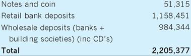
Source: Adapted from ONS (2010) Financial Statistics, September.
with building societies. Table 20.1 shows the total amounts outstanding for the different components of M4 as at August 2010.
The Divisia Index
M4 items are simply summed to give a measure of the money supply. Each item in the aggregate has a weight of unity and so all assets are weighted equally. This approach takes no account of the ‘moneyness’ of the different assets. Thus notes and coin in circulation are treated in exactly the same way as interest-bearing time deposits and any substitution of one for the other has no effect on the measured magnitude of M4. However, notes and coin function as a ‘pure’ medium of exchange and are non-interest bearing, unlike interest-bearing deposits which function primarily as a store of value. The latter earn an explicit rate of return and, at different times, switching between assets is apparent. The implicit assumption of simple sum measures of the money supply, namely that all components are perfect substitutes, is therefore erroneous.
A different approach is to weight the different assets in the money stock according to their role in transactions, i.e. according to the extent to which they function as a medium of exchange. This is the reasoning behind the Divisia Index which is claimed to be more closely related to total expenditure in the economy than conventional money aggregates. There are, of course, problems as to which variables to include in such a Divisia Index and the weight to be accorded to each variable. In practice, the basic approach has been to weight each component according to the difference between its interest yield and the yield on a safe benchmark asset. In a Divisia Index, notes and coin therefore have a weight of 1, while high-interest-bearing savings accounts have a weight closer to zero, because the interest paid on them approaches the benchmark market rate and switching into and out of such accounts makes them less useful as a measure of the medium of exchange function.
The money supply process
The creation of deposits
The existence of a legal definition of money enables us to focus on an important question: how is money created? The answer is not self-evident. Notes and coin are, of course, issued through the Bank of England and the Royal Mint, but they are not released without limit. If they were they would quickly lose value and would become unacceptable as a medium of exchange. However, before we focus on the importance of changes in base money (which includes notes and coin) in the money supply process, let us look at the creation of bank deposits. Even a cursory glance at the data for M4 in Table 20.1 shows that bank deposits are a significant component of broad money aggregates such as M4.
In any discussion of the creation of bank deposits, it is customary to begin by recognizing that not all of the funds deposited with a bank will be withdrawn at any one time. Indeed, under normal circumstances inflows and outflows of funds will be such that on any one day banks will require only a fraction of the total funds deposited with them to meet withdrawals by customers. This implies that the remainder can be lent to borrowers. But this is not the end of the story because funds lent by one bank will flow back into the banking system; again, a fraction will be retained and the remainder will be available for lending to other borrowers. This process is known as the money supply multiplier.
The money supply multiplier
Models of the money supply multiplier link the money supply to the monetary base in a relationship of the following form:
M = mB where M = the money supply;
m = the money supply multiplier;
B = the monetary base.
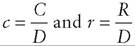
In models such as this, m tells us how many times the money supply will rise following an increase in the monetary base. But what determines the value of m? In fact, there are two factors: the decisions of depositors about their holdings of currency and deposits, and the level of reserves the banks hold to meet customer demands for currency. For simplicity, let us assume that c is the desired ratio of currency (C) to total deposits (D) and that r is the desired ratio of reserves (R) to total deposits (D). Thus we have:
Since B = C + R and M = C + D, it follows that:

which, after dividing the right-hand side by D, can be written as:
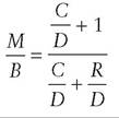
Replacing C/D with c and R/D with r we have:

Since m = M/B we can say that the money supply multiplier is determined by the public’s desired ratio of cash to total deposits (c) and the bank’s desired ratio of reserves to total deposits (r).
Whether the money supply multiplier is an adequate explanation of the money supply process depends partly on the stability of the ratios c and r. For the UK, the evidence suggests that c, the ratio of the public’s demand for cash to deposits, can be unstable and unpredictable. Of course, there are bound to be seasonal variations and it might be expected that over the Christmas period and during the summer months when more holidays are taken, the c ratio will rise because of an increase in the public’s demand for cash. However, empirical studies of the c ratio have concluded that the instability it exhibits arises for many reasons and changes do not always coincide with predictable changes in the seasons. One reason why the c ratio might be unstable is that changes in the rate of interest change the opportunity cost of holding cash. This is especially important because of the emergence of interestbearing current account deposits. Whatever the reasons, for the UK it has been estimated that the c ratio varies between 0.16 and 0.21.
The empirical evidence on the stability of the r ratio is not so conclusive and some studies suggest that r is unstable while others suggest that it is relatively stable. Again, in the short run at least, changes in the rate of interest are likely to cause changes in the r ratio. For example, when interest rates are rising, banks have an incentive to reduce their holdings of reserves.
Certainly the general view for the UK is that the money supply multiplier is unstable, at least in the short run.
The rules versus discretion debate
The rules versus discretion debate is one of the most enduring issues in monetary policy. It focuses on whether monetary policy should be conducted according to established rules, known in advance to all, or at the discretion of policy-makers. In the early years of the debate, it was argued that the case for discretion in policy rested on the view that wages and prices adjust slowly in response to shocks such as a sharp increase in the price of oil. The slow adjustment of the economy results in lost output and unemployed resources. An activist policy allows freedom to vary policy in order to speed up adjustment and move the economy towards full employment or away from inflation. The counter-argument was that discretion succeeded only in raising the long-run rate of inflation and that a policy rule, such as a constant rate of growth for the money supply, facilitated a more effective adjustment and promoted a more stable economy.
The debate has now moved on and it is accepted that if economic outcomes (such as the rate of inflation) depend on expectations about future policies, then credible pre-commitment to a rule can have favourable effects on the economic outcomes that discretionary policies cannot have. In other words, a credible rule can influence expectations and in so doing can deliver more favourable outcomes than are possible when the authorities initiate discretionary changes in policy.
To understand how this can happen, imagine if the authorities announce a target for inflation for the 12-month period ahead which is below the existing rate of inflation. If the pre-commitment to deliver a lower rate of inflation is credible, that is, if it is widely believed that the authorities will adjust policy so as to deliver the target, this will influence wage and price setting to take account of the lower expected rate of inflation. As pressure on prices and wages falls, the authorities have an incentive to renege on their commitment to a lower rate of inflation, since an expansionary policy in these circumstances will boost output with little immediate impact on inflation. Economists refer to policy announcements that are subject to change as the time inconsistency problem.
The existence of time inconsistency raises a dilemma for the authorities. If their policy announcements are not deemed to be credible, they will have no effect on expectations and it will therefore be more difficult to deliver the target outcome without reducing output and increasing unemployment. Any policy that is not time consistent will therefore be unable to deliver favourable policy outcomes, that is, low inflation at a low cost in terms of output and unemployment. However, if the authorities pre-commit to a credible policy, favourable outcomes follow naturally because of the effect the pre-commitment has on inflation expectations. In other words, announcing a rule and sticking to it delivers favourable outcomes that cannot be achieved when the authorities exercise discretion.
This conclusion is now widely accepted, but several questions immediately present themselves: what should be the ultimate goal of policy, what variable should the authorities target to achieve their goal and how can they enhance the credibility of precommitments to the target? The first of these questions is easily answered. For most central banks, the overriding priority is to maintain low and stable inflation. It is well known that inflation imposes costs on the economy in terms of resource misallocation and so on, but it is also a widely held view that an environment of low and stable inflation is more likely to encourage investment and growth. The problem for central banks is therefore how best to achieve the aim, and this involves an analysis of the issues raised in the remaining two questions. We consider each in turn.
I Monetary policy targets
Monetary targeting
One of the earliest proposals for a rule, particularly associated with Milton Friedman, was to establish a monetary rule. Such a rule involves setting a target rate of growth for the money supply. Monetary targeting can be analysed within the quantity theory framework. For example, if over some given period, Vy is expected to fall by 1%, the target rate of inflation is 2% and Y is expected to grow by 21%, the quantity theory predicts that the inflation target will be achieved if the money growth target is fixed (and achieved) at roughly 52%.
In fact, it is no longer thought that inflation can be controlled directly by setting target rates of growth for the money supply. This does not necessarily imply that the quantity theory of money does not predict a causal link from money to prices. The predictions of the quantity theory are much more reliable in the long run, but over the medium term the relationship between money and prices is less precise. Because of this, as the following discussion shows, there are severe problems with monetary targeting and with interpreting the components of the quantity theory of money.
Problems with monetary targeting
Our simple example above assumes that variables in the quantity theory equation can be accurately measured. In reality the growth of output depends on the availability of factors of production and their productivity. These are very difficult to measure and forecast, especially if an economy is undergoing structural change. In the UK in the 1980s and 1990s, structural changes occurred because of privatization and deregulation, trade union reform and so on. In the early years of the new millennium other structural changes are taking place, such as the rising number of schoolleavers entering further and higher education rather than the labour market.
It is also unclear which definition of money most accurately captures the causal link from money to prices. Narrow definitions of money are more easily controlled, but they omit some liabilities of the banking system that have an important bearing on inflation. Divisia attempts to weight the various components of any definition of money according to their impact on prices. However, identifying appropriate weights has proved problematical and there is no agreement that Divisia offers any advantages over more conventional measures of money.
Deregulation and development of the financial sector have also caused problems in predicting velocity of circulation. Financial deregulation usually results in a permanent reduction in velocity of circulation of broad money. To the extent that this happens, an increase in broad money growth might not imply an increase in the future rate of inflation. If there are frequent and unexpected changes in velocity, pursuing an inflexible money growth target can cause short-run swings in interest rates and real output as demand for money changes but supply of money does not respond.
Another problem with monetary targeting is that even if velocity is stable in the long run, short-run changes in velocity will cause unanticipated changes in interest rates. A change in velocity implies a change in demand for money and, with supply changing according to some fixed rule, interest rates will adjust in order to maintain equilibrium between demand for money and supply of money. Such unanticipated changes in interest rates will adversely affect investment and might have other adverse consequences on the economy through their effect on the exchange rate.
Exchange rate targeting
An exchange rate target simply involves fixing the external value of one currency against another, low- inflation, currency. Over time this will result in the prices of tradeable goods and domestic inflation converging towards foreign levels. Maintaining the fixed exchange rate implies that domestic monetary policy must follow the monetary policy of the anchor currency, otherwise there will be pressure on the exchange rate.
A major advantage of exchange rate targeting over monetary targeting is that unanticipated changes in money demand have no effect on domestic interest rates because they will be matched by an equivalent and offsetting change in money supply through capital flows. Exchange rate targets are also transparent and easy for the general public to understand. To the extent that exchange rate targets are credible, they therefore provide information on which expectations can be based. The major problem with exchange rate targets is that they leave the authorities powerless to deal with adverse shocks to the economy, such as a deterioration in the terms of trade or a loss of export markets. Unless wages and prices are flexible, an adverse shock must be borne by the domestic economy and will result in declining output and rising unemployment. This will continue until the economy slows up sufficiently and wages and prices fall far enough to restore competitiveness.
Inflation rate targeting
When the authorities target the rate of inflation, the simplest case is when monetary policy is adjusted whenever the forecast rate of inflation rises above the announced target range. If inflation is above the target range, monetary policy is tightened and vice versa. However, central banks that target the rate of inflation have generally adopted a broader approach and, as well as monitoring forecast changes in the rate of inflation, also look at other factors: the overall state of the economy, rates of wage change and so on.
This is a much more flexible approach than a rigid monetary rule. It gives the central bank scope to respond to unanticipated shocks or cyclical changes in the economy which might require an easing or tightening of monetary policy to avoid some adverse effect on the economy. For example, if there is a downturn in economic activity which might develop into a recession, the central bank can cut interest rates to reduce the possibility of this eventuality. In adopting an inflation target which is to be interpreted flexibly, the central bank has some freedom to manoeuvre and is able to respond flexibly to changing circumstances without compromising its inflation target.
To see the advantage of this, consider the effect of a demand-side shock and a supply-side shock. When the economy is subject to a demand-side shock, output and inflation rise and fall together. For example, if there is a sharp fall in the demand for exports, inflation and output fall. In such cases, the optimal response of the central bank is clear and monetary policy should be loosened. Supply-side shocks, on the other hand, move the economy in opposite directions. For example, a sharp rise in the price of oil would push up input prices and would inject an inflationary impetus into the economy. Simultaneously the higher price of oil causes a reduction in aggregate demand and a consequent fall in output and employment. In this case, the bank has to decide on the optimal response. Either it can bring inflation down rapidly by a sharp tightening of monetary policy so that the burden of adjustment falls entirely on output, or it can tighten monetary policy less severely so that the burden of adjustment is shared between prices and output. By changing the policy time horizon, the time by which inflation should be back within the target range, the central bank spreads the output consequences of reducing inflation over a longer time period, thereby reducing the impact on employment, rather than compressing it into a shorter time horizon. Figures 20.6(a) and (b) illustrate the point.
In Figs 20.6(a) and (b), AD and AS are the original aggregate demand and aggregate supply curves. The price level is initially P and output is Y. In Fig. 20.6(a), an unanticipated fall in aggregate demand shifts the aggregate demand to AD1. As a result prices fall to P1 and output falls to Y1. In this case, the appropriate response of the authorities is to loosen monetary policy and so move aggregate demand back towards its original position. In Fig. 20.6(b), there is an unanticipated adverse supply shock which reduces aggregate supply to AS1. In this case the bank has a range of policy responses depending on its priorities. It can tighten monetary policy severely enough so that aggregate demand and, through this, output fall far enough to preserve price stability (Y2). Alternatively, it can loosen monetary policy far enough so that output is unchanged but prices are given a further upward twist (P2). Between these two extremes there exist an infinite number of policy choices which result in the burden of adjustment being shared between output and prices. The distribution of the burden depends on the preferences of the central bank.
I Central bank credibility
Central bank credibility refers to the degree of confidence the public has in the central bank’s
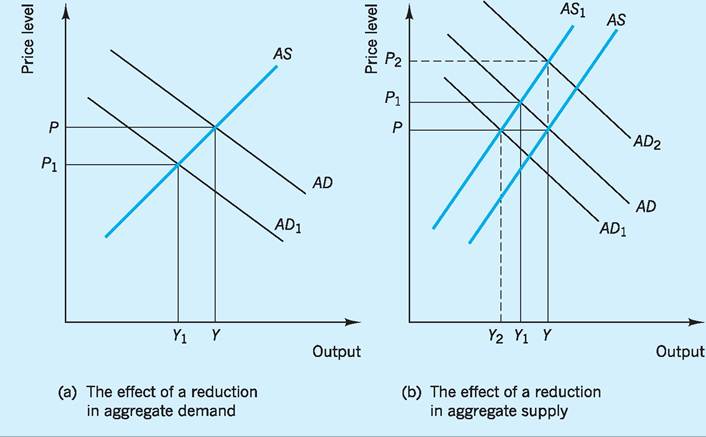
Fig. 20.6 The effects of reductions in aggregate demand and supply.
determination and ability to meet its announced targets. In reality, establishing credibility can sometimes be difficult because, as we have argued above, there are incentives for policy-makers to default on commitments that are widely believed. So how can credibility be improved and maintained?
In establishing and maintaining credibility, the overriding priority is that the authorities must be able to persuade the public that there is no inconsistency between their policy objectives. If policy objectives are inconsistent, any attempt to establish credibility will fail. Most central banks currently emphasize their commitment to price stability as their primary aim and promulgate the view that other aims, such as high and stable levels of employment, will be pursued only to the extent that they do not jeopardize price stability.
There would not seem to be any inconsistency in these objectives, but credibility will be more easily established and maintained in a stable economic environment in which the target rate of inflation is consistently delivered. If there is an economic downturn that monetary policy is unable to correct, it is possible that as unemployment rises the public might form the view that the government will reconsider its policy stance. To the extent that this creates the expectation of a higher rate of inflation, central bank credibility will be compromised. The old adage that ‘nothing succeeds like success’ is also true of central bank credibility. When the economy is performing well and the central bank is delivering its targets, credibility will be easier to establish than when the economy is not performing well.
As noted above, there are lags before changes in monetary policy take effect. In the meantime, inflation might be subject to change because of unforeseen events that make control in the short term difficult. Yet the central bank will be judged by outcomes, and where these differ from the central bank’s announced targets, its credibility might be damaged. The central bank can minimize the damage by ensuring that the public is fully informed of events and why the measures it has taken are consistent with the announced policy objective.
Transparency in monetary policy
Central bank credibility is far easier to establish when policy is transparent. With respect to monetary policy, transparency is important whenever there is incomplete or imperfect information. Information might be incomplete or imperfect with respect to:
■ the central bank’s objectives;
■ understanding the links between policy changes and the central bank’s objectives; and/or
■ the information the central bank has available on which to base policy changes.
We consider each in turn.
The central bank's objectives
As far as the objectives of the central bank are concerned, transparency involves more than the central bank simply stating its objectives. The public might be uncertain about the true nature of the objectives or the extent to which the central bank will trade off one objective (inflation) against another objective (unemployment). Transparency with respect to objectives requires the central bank to pursue clear objectives for aggregates which are familiar to the public. The public can then readily observe the behaviour of these target aggregates and judge for themselves the extent of transparency. Transparency is most likely to be achieved when the objectives of the central bank are either enshrined in its constitution or imposed on it by government. Currently many central banks pursue an inflation target (see p. 410). In some cases, such as the European Central Bank (ECB), the target value for inflation is set out in their constitution. In other cases, such as the Bank of England, the target rate of inflation is set by government.
The role of policy changes
Even if the central bank’s objectives are clearly understood, transparency is not guaranteed, since the public might not understand the operation of the techniques used to achieve the target. For example, if the main policy instrument is interest rates, how big a change in interest rates is required each time the projected value of inflation deviates by x% from its target rate? Little can be said about this, since the relationship is imperfectly understood even by economists! What we can say is that transparency will be easier to achieve if interest rates move predictably in response to projected deviations in the rate of inflation from target.
The importance of information
The public might understand the central bank’s objectives and the expected behaviour of interest rates in response to projected values for the rate of inflation, yet policy transparency might still not be achieved if the public do not have access to the same information as the central bank. For example, if the central bank has access to information that implies a slowdown in the economy and a significant reduction in the rate of inflation, the expected policy response would be a cut in interest rates. However, if the public do not have access to the same information they might misunderstand the motives behind the cut in interest rates. Ignorance of the expected recession might lead the public to form the erroneous view that policy was jeopardizing the inflation objective.
In reality, lack of information might not pose a serious problem if the public are informed of the reasons behind monetary policy decisions. It is for this reason that many central banks publish minutes of their monetary policy committee meetings. These minutes explain the information on which policy changes are based and the reasons for the particular extent of the policy change. Other information is often also made available to the public, such as the Inflation Report published by the Bank of England which details the bank’s forecast of inflation for the period ahead.
Techniques of monetary policy
Over the years, a variety of techniques have been used to implement monetary policy. However, we can group the techniques of monetary policy into two broad approaches: those which impose direct controls on the banking sector and market-based instruments which focus on interest rates. Both have been used by the Bank of England (as well as other central banks) to implement monetary policy.
Direct controls
Direct controls focus on the growth of bank deposits and often involve legal measures specifying that financial institutions are required to hold part of their assets in a defined form such as cash or other liquid assets, usually referred to as reserve assets. The central bank can then seek to control the growth of bank deposits by limiting the availability of reserve assets. There are two main ways in which this can be done.
1 Special deposits. One technique used in the past was to impose special deposits on the banking sector. These deposits were ‘frozen’ at the central bank and the banking sector had no access to them (although they continued to earn interest at the treasury bill rate) until they were released by the central bank. A call for special deposits implied a reduction in the banks’ operational deposits at the central bank and this again put pressure on the banking sector to reduce its lending. This technique was abandoned in 1971.
2 Credit ceilings. The central bank has also used credit ceilings, known as supplementary special deposits, to limit the growth of bank lending. These were imposed on the banking sector when their liabilities (bank deposits) rose above a specified level. In such cases, banks were required to make non-interest bearing deposits with the central bank in proportion to the growth of their liabilities. This technique was abandoned in 1980.
The principal advantage of direct controls is that they provide the central bank with a way of controlling the quantity or maximum price of credit. This might be particularly useful in a temporary crisis. They might also provide the only practicable way to implement monetary policy when financial markets are undeveloped. However, there are severe problems associated with these direct techniques of monetary control. Probably the major disadvantage is that they tend to be ineffective because they encourage disintermediation, that is, the diversion of business away from the regulated sector to unregulated sectors of the economy. This must be inefficient because if the unregulated sector was operating efficiently, it would already be providing a greater proportion of the business provided by the regulated sector! When direct controls are in place, savers and borrowers search for ways of circumventing the regulations. One obvious route through which regulations at home can be bypassed is by transferring business abroad. Regulations are also inefficient because they tend to stifle competition between banks and limit the benefits to borrowers and depositors.
Indirect controls
Indirect controls exert their influence through channels that leave the financial institutions free of direct controls (other than those necessary for prudential control of the banking system). Reserve asset ratios were abolished in 1981 and in more recent years the Bank of England has exercised control by measures which focus on the availability of base money (notes and coin held by the banking sector plus reserve balances at the Bank of England). Again these might take a variety of forms.
■ Reserve requirements. Reserve requirements impose restrictions on the form in which banks must hold their assets. They usually involve a requirement that total assets can be no greater than the maximum value of some defined group of assets (reserve assets). For example, if reserve assets are defined as the monetary base, then total assets can be no greater than some multiple of the monetary base.
■ Funding. During the 1980s, the Bank of England exerted its influence on the banking sector by funding the national debt. This technique involved the Bank in issuing fewer short-term securities and more long-term securities. Because treasury bills constituted part of the liquid assets ratio but longterm securities did not, the aim was to leave the banks short of liquid assets and compel them to cut their lending.
■ Interest rates. The Bank of England has considerable influence over short-term rates of interest because of the role it performs in the domestic money markets. As banker to the government and to the banks, it is able to forecast fairly accurately the daily flows of funds between the government’s account and the accounts of the banks. When more money flows from the banks’ accounts to the government’s account the market will be short of funds; when funds flow in the opposite direction, the market will have a surplus of funds. The Bank of England operates on a daily basis to smooth these flows of funds but tends to conduct its openmarket operations (see p. 444) in such a way as to leave the market short of funds. It then relieves this shortage by lending to the different institutions at a repo rate (official rate) of its own choosing. For example, if the Bank of England sells gilts (government bonds) in the open market there will be a transfer of deposits from the banks’ operational balances at the Bank of England into the government’s own account as cheques authorizing payment are cleared. As operational balances fall, banks are forced to borrow from the Bank of England.
Rather than dealing with every individual bank, the Bank of England uses the discount houses as an intermediary. The discount houses have borrowing facilities at the Bank of England and, when the market is short of funds, the discount houses are ‘forced into the Bank’. The Bank of England provides them with cash either by re-discounting bills held by the discount houses or by lending direct. When the Bank changes the rate implied in the price at which it rediscounts bills or the repo rate at which it lends, all institutions quickly follow the Bank’s lead and adjust their own rates of interest.
Central banks in developed economies rely almost entirely on indirect controls. Such controls are effective because they are non-selective and affect all institutions across the entire spectrum. For example, when the Bank raises its minimum lending rate (discount rate) this will affect all institutions indiscriminately and will result in interest rates rising throughout the economy. Indirect controls therefore avoid these problems associated with direct controls but are not as flexible as they might seem. Interest rates can be changed quickly, but the Bank of England estimates that it can take up to two years for a change in interest rates to exert its full impact on inflation.
UK monetary policy since the 1950s
Monetary control in the 1950s and 1960s
In the 1950s and 1960s the Keynesian view of money was the consensus view. There was a widespread belief that money growth exerted its influence on the economy through changes in the rate of interest which stimulated changes in the rate of investment. However, monetary policy was viewed as having a weak effect, since the available empirical evidence strongly suggested that investment was interestinelastic. The prevailing view was that investment by firms in fixed assets and stocks, if it was influenced at all by monetary factors, was influenced more by the availability of credit rather than by its nominal cost.
Consequently monetary policy consisted primarily of ceilings on lending, although open-market operations and special deposits were also used during this period.
Competition and Credit Control (CCC), 1971
In 1971 the focus of monetary policy switched decisively. Interest rates were, ostensibly at least, to be market determined rather than imposed by the authorities. Furthermore, regulations were introduced compelling banks to observe a minimum 12.5% reserve assets ratio between eligible reserve assets and eligible liabilities. The former were defined as private-sector non-bank deposits and building society deposits. The latter included balances at the Bank of England, money at call and short notice with the discount houses, British government and Northern Ireland treasury bills, local authority bills and commercial bills eligible for rediscount at the Bank.
Whenever eligible reserve assets fell below the 12.5% minimum level, it followed that banks would be compelled to reduce their lending. Whenever it wanted to tighten monetary policy, the Bank of England could always engineer such an event, for example by calling for special deposits. In reality, although rates of interest were supposed to be market determined, the Bank of England frequently intervened to leave the banks short of funds, leaving it free to adjust interest rates.
Competition and Credit Control was in place for less than a decade. It failed to provide an effective framework for monetary policy for a variety of reasons. For example, it was unclear whether interest rates were market determined or whether the authorities were setting interest rates. (We have already argued that there are clear benefits arising from transparency.) Probably of more significance is that the regulations applied only to defined institutions and there was an explosion of growth in the unregulated sector. Rising inflation in the 1970s also caused problems because it led to rising public-sector borrowing and, rather than disrupt long-term interest rates through funding, the government borrowed short-term thus ensuring an adequate supply of liquidity to the banking sector. Despite these problems, it was the abolition of exchange controls in 1979 that finally brought the framework to an end.
Capital flows between countries increased (see Chapter 26) to the extent that effective monetary control became impossible, since residents were enabled to open overseas bank accounts and to borrow abroad for current spending in the UK.
The medium-term financial strategy (MTFS), 1980
In March 1980 the government unveiled its new approach to monetary control, the medium-term financial strategy (MTFS). The MTFS was designed to provide a framework of control within which money growth could be targeted over a four-year period. The emphasis of control shifted in two ways:
1 from a short-term to a medium-term perspective; and
2 from controlling the availability of reserve assets to controlling the growth of bank assets, the so-called ‘counterparts’ to the money stock.
The rationale for shifting to a medium-term perspective is an admission that it is impossible to exercise control over money growth over a short time horizon. The rationale for controlling the counterparts to the money stock reflects the fact that, apart from the narrowest measures of money, definitions of the money stock focus on bank deposits. There is a famous banking maxim that ‘every loan creates a deposit’ because every loan granted by a bank is redeposited within the banking sector after being spent by the borrower. Controlling the counterparts of the money stock was therefore seen as a way of controlling money growth. In the UK, the authorities attempted to control growth of the (now defunct) broad measure of money known as sterling M3 (£M3). The MTFS set declining target rates of growth for £M3 annually so that as one year in the four-year cycle passed, another year began.
Bank deposits consist of lending to the government, the private sector and the overseas sector. The sum of lending to each of these forms the counterparts to the money stock, and the MTFS included specific measures to control each of these individually.
■ Government expenditure was to be progressively reduced to rein back the PSBR (now PSNCR). This was made easier because the proceeds from privatization were treated not, as might be expected, as a means of financing the PSBR, but as a means of reducing it!
■ Debt sales to the non-bank private sector were encouraged by adjusting interest rates to the level required to persuade the non-bank private sector to take up offers of treasury bills.
■ Exchange rate policy was to be used to influence the external and foreign currency counterparts of the money stock.
Additional measures, designed to improve the effectiveness of monetary control by addressing some of the problems associated with Competition and Credit Control, were introduced in August 1981. Thenceforth banking regulations applied to all monetary institutions within the monetary sector. This is to avoid the emergence of disintermediation. The reserve assets ratio was abolished and a minimum figure (now abolished) was established for operational deposits.
The MTFS proved no more effective as a framework for monetary policy than did Competition and Credit Control. Monetary growth frequently exceeded the target growth rate and, in an attempt to improve control, target rates of growth for the then monetary base (M0) were introduced in 1984. By 1987 targets for £M3 were abandoned, although the Bank of England continues to ‘monitor’ changes in M0. There are many reasons why it proved difficult to restrain £M3 within its target range. One reason is that private-sector borrowing proved less sensitive to rising interest rates than anticipated. However, the main reason is that deregulation of the financial sector and product innovation distorted the money aggregates to the extent that they became unreliable as indicators of money growth.
Exchange rate and inflation rate targeting
As confidence in the efficacy of targeting money growth waned, the authorities turned to the exchange rate as an anchor for monetary policy. In the late 1980s sterling shadowed the Deutsche mark (DM) before the official announcement in October 1990 that sterling was to join the ERM at a rate of £1 = DM2.95. It soon became clear that at this exchange rate sterling was hopelessly overvalued on the foreign exchanges, and in September 1992, with the UK deep in recession and interest rates at 15% to preserve the exchange rate, the Chancellor of the Exchequer bowed to the inevitable and withdrew sterling from the ERM. The following day interest rates were reduced to 10% and, free of exchange rate constraints, the focus of policy changed.
In October 1992, the Chancellor announced that monetary policy would henceforth target the rate of inflation. The first steps towards increasing transparency and credibility quickly followed when, later the same month, the Chancellor announced that the Governor of the Bank of England would produce a regular report on progress towards the inflation target. The Inflation Report is compiled by the Bank in the belief that it will be more credible than if it is produced by the government. In 1994, transparency was further increased when it was announced that minutes of meetings between the Chancellor and the Governor of the Bank of England to review the performance of monetary policy would be published. The Inflation Report and the Minutes of the Monetary Policy Committee (MPC) meetings (see below) remain an important mechanism through which the Bank communicates its views and actions to the general public.
The inflation target was initially set in the range 1-4% per annum, but in 1997 a point target of 2.5% for RPIX inflation was introduced. This was subsequently revised on 10 December 2003 to a point target of 2% for CPI inflation, and the target rate of inflation for the UK remains at this level. In principle, inflation targets are easy to understand: the central bank simply adjusts policy (usually its discount rate - i.e. the minimum lending rate in the UK) whenever forecast inflation rises above or falls below the target rate. In practice, all central banks face constraints on their ability to take action whenever forecast inflation deviates from the target. For example, in September 2010, inflation in the UK on the CPI measure (the government’s target measure) was 3.1%, yet on 7 October the Bank of England announced that it was leaving the minimum lending rate unchanged at 0.5%, where it has been since March 2009. The problem is the depressed and fragile nature of the UK economy which some analysts predict is on the verge of a second recession. An increase in interest rates would further depress aggregate demand and increase the likelihood of another recession or, even worse, it might send the economy into a deflationary spiral.
The main advantage of an inflation target over, say, a monetary rule where the money supply grows by a fixed amount, is that it gives the Bank flexibility to respond to adverse shocks, whether these are anticipated or unanticipated. An anticipated shock of a sufficient magnitude would simply trigger a coun- terfactual change in interest rates before the shock materialized, whereas an unanticipated shock of a sufficient magnitude would trigger a counterfactual change in monetary policy at the first opportunity. With respect to the Bank of England, this would be at the next meeting of the MPC.
Operational independence of the Bank of England
In furtherance of the aim of achieving credibility, on 6 May 1997, the Bank of England was given operational responsibility for setting short-term interest rates to achieve the inflation target, initially retained by the Labour government at 2.5% but revised downwards in 2003 to 20%. However, the incoming Chancellor, Gordon Brown, made it clear that the government would retain a national interest in controlling inflation. This is effectively an escape clause allowing it to overrule the Bank’s interest rates decisions in pursuit of the inflation target when it deems such action necessary. Neither the Labour government nor the post-2010 Coalition government has specified any formal process for implementing the escape clause, nor defined a set of conditions under which the Bank would be overruled. Nevertheless, the point target now has a one percentage point threshold either side and if inflation breaches this, the MPC (which decides on interest rate changes, see below) is required to publish an open letter outlining the reasons for the deviation and to explain the policy changes to be adopted so as to bring inflation back to target.
The MPC, with a membership of nine and a quorum of six, meets monthly at the Bank of England to decide on the timing and extent of any change in the rate of interest for the month ahead. The broad aim is to keep the growth of demand in line with supply-side capacity as reflected by consistently low inflation. Subject to the primacy of hitting the inflation target, the MPC is required to support the government’s economic policy, including its objectives for growth and employment. Monetary policy is therefore loosened or tightened in order to moderate the fluctuations that occur over the business cycle. It is anticipated that the target rate of inflation is consistent with delivering steadier growth, higher levels of employment and rising living standards into the medium and longer term.
The making of monetary policy in the UK
The making of monetary policy in the UK follows a clearly defined monthly cycle. Decisions are taken by a simple majority vote. The timetable for a typical monthly round of the MPC is set out in Table 20.2.
Recent developments in UK monetary policy
UK monetary policy in recent years has focused on tackling deflation, especially by injecting more money into the economy via quantitative easing and keeping interest rates at extremely low levels.
Deflation
The primary economic aim of the Bank of England is to maintain a low and stable rate of inflation with a target rate of 2%. Since the 1980s, relatively high inflation has been more of a problem for the UK than relatively low inflation, but in more recent years in the UK, as well as Europe and the US, the prospect of deflation has caused concern. Deflation differs from disinflation which simply means a fall in the rate of inflation. Deflation actually implies falling prices and has potentially serious consequences for the economy. It is to counter the prospect of deflation that the Bank of England (and the Federal Reserve in the US) has introduced its quantitative easing programme. Before we discuss the nature of quantitative easing, we briefly consider the causes and consequences of deflation.
Sources of deflation
Economists generally agree that in the long run inflation and deflation are monetary phenomena. In this sense, deflation is caused by a reduction in aggregate demand that is so severe that traders are obliged to persistently reduce prices to help retain sales volume. Some economists have argued that the expenditure cuts announced by the new Coalition government in October 2010 are so severe that they might trigger deflation (see Chapter 18). Of course, other mechanisms might trigger deflation; even a positive supply shock to labour productivity can put downward pressure on prices, as nominal wage rates adjust only slowly upwards to unexpected increases in output, so that as output per hour rises faster than hourly wage rates, unit labour costs decline and in competitive markets prices fall. If the productivity shock is widespread, its effect might be to drive the price level downwards. Falling prices in some sectors might also impact on other sectors as lower inflation induces lower wage rises, which in turn generate lower inflation, and so on until the price level begins to fall.
Table 20.2 Typical monthly round of the MPC.
Briefing
| Throughout the month | Circulation of briefing material and analysis of data releases and market developments by staff |
| Friday before policy meeting Monday/Tuesday | Half-day pre-MPC meeting Staff undertake follow-up work requested by the Committee |
| Policy meeting Wednesday | Policy meeting commences early afternoon. Committee identifies the key issues and debates their implications for inflation prospects |
| Thursday | Policy meeting concludes. Committee members provide their assessment of the appropriate policy stance and vote on the level of interest rates. Policy announcement at noon. Decision implemented immediately in a round of open-market operations at 12.15 |
| Minutes Week following policy meeting | Draft of the Minutes circulated and comments from Committee Members incorporated |
| Monday (second week after policy meeting) Wednesday (two weeks after policy meeting) | Committee meets and signs off the Minutes Publication of the Minutes at 09.30 |
Source: Bean and Jenkinson (2001).
Problems with deflation
Problems with deflation include the following.
■ Misallocation of resources. Governments and policy-makers worry about deflation for the same reasons they worry about inflation. Like inflation, deflation impairs the ability of the price mechanism to allocate resources efficiently since it blurs the distinction between absolute and relative price changes. When demand for a product changes, prices rise or fall and this leads to changes in output to accommodate the change in demand. However, the price mechanism can only discharge its role efficiently if suppliers are able to distinguish between a change in the price of a single product and a change in the average price of all products (the price level). This is not as easy as it seems because, during periods of inflation or deflation, not all prices change by the same amount, at the same time or even in the same direction! During inflation some prices actually fall, and during deflation some prices actually rise. It is the general price level that changes. When producers fail to distinguish between a change in the price of a single product and a change in the average price of all products they misread the information contained in price signals and adjust output in ways which are often contrary to changes in demand. The result is then a misallocation of resources in the economy which results in the over-production of some goods and the under-production of others in relation to the optimum level of output.
■ Postponement of spending decisions. Other problems with deflation result from it creating incentives to save and to postpone spending, because prices will be lower and purchasing power greater in the future. Deflation can be extremely damaging when people postpone spending in the anticipation of cheaper future prices, as this depresses current spending and, as stocks accumulate and profits fall, firms cut back on production and on employment and cut prices. The longer consumers postpone their spending, the longer and more pronounced the deflation will be.
■ Borrowers lose out. Deflation also worsens repayment burdens for borrowers because debts remain fixed in nominal terms (for each £100 borrowed, £100 must be repaid), but wages and prices fall during deflation. This not only causes hardship for individual households, but also causes problems for firms who will cut back on borrowing and investment as debt repayment burdens increase. There is also likely to be a greater number of defaults on loans and the banking sector is therefore likely to restrict lending, making recovery from deflation still more difficult. This has certainly been a factor in the ongoing problems faced by the Japanese economy.
■ ‘Zero bound’ and policy-making problems. For policy-makers, a major problem associated with deflation is that posed by the so-called ‘zero bound’. A major determinant of nominal interest rates is expected inflation, and since prices fall during deflation, nominal interest rates also tend to fall. However, once the nominal interest rate is at zero, no further downward adjustment in the rate can occur, since lenders will not accept a negative nominal interest rate when it is possible instead to hold cash. At this point, the nominal interest rate is said to have hit the ‘zero bound’. This poses a major problem because when the nominal interest rate has been reduced to zero (as in the US), the real interest rate paid by borrowers equals the expected rate of deflation. For example, if deflation is at an annual rate of 2%, then someone who borrows for a year at a nominal interest rate of zero actually faces a 2% real cost of funds, as the loan must be repaid in pounds sterling whose purchasing power is 2% greater than that of the pounds borrowed originally. In a period of sufficiently severe deflation, the real cost of borrowing becomes prohibitive. Capital investment, purchases of new homes and other types of spending decline accordingly, accelerating still further the economic downturn.
The zero bound also places severe limitations on the conduct of monetary policy. Under normal conditions, the Bank of England (and most other central banks) will implement policy by setting a target for a short-term interest rate and enforcing that target by buying and selling securities in open capital markets (open market operations). When the short-term interest rate hits zero, the central bank can no longer ease policy by lowering its usual interest-rate target. The central bank’s inability to use its traditional methods for conducting monetary policy at the very least complicates the policy-making process and introduces uncertainty as to the size and timing of the economy’s response to policy actions. One thing we have learned about monetary policy in recent decades is that it operates more efficiently when it is predictable!
In the UK, interest rates have been close to the zero bound since March 2009, but with output growing only slowly (0.8% in the third quarter of 2010) and unemployment forecast to rise sharply, the Bank’s options to stimulate the economy are limited. For this reason, the bank has implemented quantitative easing which simply means that it injects more money into the economy with the aim of stimulating demand. This implies that the Bank at least partly believes that the velocity of circulation will not decrease so as to fully offset the stimulus that increased money supply growth will bring. The extra money supply is created by the bank buying assets, primarily gilts.
Quantitative easing
Quantitative easing (QE) refers to the process through which the central bank injects more money into the economy (see Fig. 20.7). It does this through asset purchases, primarily gilts, in the open market. As purchases of assets increase, the amount of cash and liquidity in the economic system increases, stimulating spending and creating a ‘wealth effect’, as the extra demand for assets raises their price and assetholders will experience a rise in wealth, whether they choose to sell their assets or retain them! Higher wealth might encourage additional spending and, to the extent that this does happen, it will reinforce the effects of QE. Higher asset prices also mean lower yields, with the new lower effective interest rates making it cheaper to borrow to finance spending. As banks receive cash from selling their assets to the central bank, their operational deposits with the Bank of England rise and they can use these to stimulate further lending to their customers via the money supply multiplier (p. 407).
However, it is possible that the financial crisis will have left banks nervous and reluctant to increase their lending. It is for this reason that the Bank of England is particularly targeting the wider economy and purchasing mainly in private-sector asset markets, in other words purchasing private-sector assets, mainly from non-bank asset-holders. By reassuring the markets of its willingness to buy debt, the Bank’s intention is to encourage lending, since its actions guarantee a ready market for assets if financial intermediaries, firms or individuals experience a tightening of their liquidity situations. A further result of QE is that as asset prices rise, interest rates, which move inversely with asset prices, will fall and the effect will be to encourage borrowers and stimulate spending. Figure 20.7 shows how QE works.
By early 2011 the QE programme has resulted in asset purchases by the Bank of £200bn and there is evidence that M4 has slowly started to rise. However, it remains to be seen whether this rise will be sustained and what the impact on the real economy will be. In Japan, where QE has been tried for over a decade now, the effect on the real economy has been limited - but so too has been the scale of the QE programme which was comparatively small in Japan compared to that undertaken by the Bank of England, and by the US Federal Reserve which introduced a one trillion dollar programme in March 2009.
One interesting point to note with respect to QE is that although it does not imply a return to monetarist thinking, it does imply a belief in the impact of money supply growth on aggregate spending. If increased money supply growth was not expected to generate an increase in aggregate demand, there would be no point in implementing the QE programme in the first place! While the strictest interpretation of monetarism, with its adherence to a stable velocity of circulation at its core, has not been resurrected by the QE programme, it remains clear that the Bank does not believe that a change in money supply growth will be matched by an equal and offsetting reduction in the velocity of circulation.
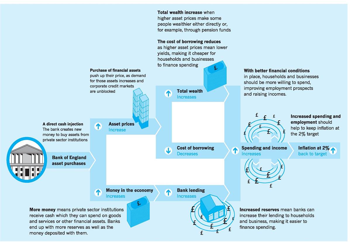
420 CHAPTER 20 MONEY AND MONETARY POLICY
Fig. 20.7 Quantitative easing. Source: Bank of England (2010).
I Conclusion
A number of conclusions might be drawn from the UK experience of money growth and monetary control since the 1980s.
1 Financial innovation and deregulation make it impossible to define a set of assets which alone function as money. This is the major reason the broad money aggregates have been subjected to continuous redefinition.
2 Controversy remains about how useful the definitions of money are. In the UK, one measure of narrow money (M0) and one measure of broad money (M4) are monitored. However, different measures of money are published in different countries and the accepted view is that when interpreting monetary conditions, definitions of money do not always include all of the relevant variables. There is also a view that weighted measures of the money stock (Divisia) might be more useful than ‘simple sum’ measures.
3 Doubt remains as to whether the direction of causation is from money to prices or from prices to money. However, growing evidence does support the view that the velocity of circulation of money follows a relatively stable trend, though there are short-run fluctuations about this trend.
4 Controlling a particular money aggregate is difficult because of financial innovation, deregulation and disintermediation. Monetary control is especially difficult because of disintermediation (see also Chapter 21).
5 The focus of monetary policy has switched from controlling intermediate variables such as the money stock or the exchange rate which were formally thought to be linked to the rate of inflation, to direct targeting of the rate of inflation.
6 Monetary policy actions focus on changes in the rate of interest which affect all institutions simultaneously and equally.
7 The adoption of quantitative easing (QE) policies is a recognition by governments and central banks of the continued effectiveness of money supply policies on the real economy, especially when interest rates are often close to zero.
Key points
■ Money functions as a unit of account, a medium of exchange and a store of value.
■ Money avoids the inefficiency of a barter system, permitting greater specialization and associated scale economies.
■ For most purposes, M4 is the most important official definition of money and is a broad measure of the money stock.
■ Deposits at financial institutions are the most important component of broad money.
■ Definitions of money are constantly evolving because of financial deregulation and innovation.
■ Monetary policy is most effective when it is both credible and transparent.
■ Since 1992, the Bank of England has adopted an inflation target as the nominal anchor for monetary policy.
■ The Bank of England was granted operational independence on 6 May 1997.
■ There has been an increasing policy concern with avoiding deflation via monetary policy since the onset of the global recession of late 2007.
■ Governments and central banks are increasingly turning to ‘quantitative easing’ as a technique to stimulate their economies, especially when interest rate policies are restricted by ‘zero bound’ issues.
Now try the self-check questions for this chapter on the Companion Website. You will also find useful links to relevant websites.
Notes
1 It is important to understand that in arguing that velocity is stable, the monetarists are not arguing that it is constant. Instead they have always claimed that velocity changes only slowly over time and in a predictable way. In this sense it can be regarded as stable from one time period to the next. We shall see later that this has important implications for policy purposes.
2 The quantity theory states that MVy = PY. If we multiply the average price of final output by the volume of final output we obtain GNP. The quantity theory can therefore be written as MVy = GNP and hence Vy = GNP/M. The problem is which measure of money do we use? If an inappropriate aggregate for M is substituted, the value obtained for Vy will be inaccurate. Economists cannot agree on an appropriate definition of money and this has caused problems with attempts to test the stability of Vγ.
3 For example, a consol (an irredeemable bond) issued at 3% with a par value of £1m pays its owner £30,000 per annum. If the current market price of the consol is less than par, for example £0.9m, then the market rate of interest is 0.03/0.9 = 3.33%. Hence there is an inverse relationship between bond prices and the rate of interest.
4 It is sometimes argued that in the extreme a liquidity trap exists so that any change in the money supply leaves interest rates unchanged. Since the Keynesian transmission mechanism is through changes in interest rates, in this extreme situation an increase in money growth has no effect on the price level (P) or real output (Y). The increase in money growth has therefore been completely absorbed into idle balances, i.e. its effects have been offset by a reduction in the velocity of circulation. In other words, the increase in money supply is matched by an increase in the demand for money.
References and further reading
Bank of England (2010) Quantitative Easing Explained, pamphlet, London.
Bank of England Inflation Reports (various) Supplements to Bank of England Quarterly Bulletins.
Bean, C. (2002) The MPC and the UK economy: should we fear the D words? Speech delivered to the Emmanuel Society, London, 25 November 2002, Bank of England Quarterly Bulletin, Winter, 475-85.
Bean, C. (2009) Quantitative Easing: An Interim Report, speech given to the London Society of Chartered Accountants, London, 13 October 2009.
Bean, C. and Jenkinson, N. (2001) The formulation of monetary policy at the Bank of England, Bank of England Quarterly Bulletin, Winter, 434-41.
Benassy-Quere, A. and Coeure, B. (2010) Economic Policy, Oxford, Oxford University Press.
Benati, L. (2005) Long-run evidence on money growth and inflation, Bank of England Quarterly Bulletin, Autumn, 48-80.
Chote, R. (1997) Treading the line between credibility and humility, Financial Times, 13 June.
Dungey M., Fry, R., Gonzales-Hermosillo, B. and Martin, V. (2011) Transmission of Financial Crises and Contagion, Oxford, Oxford University Press.
European Central Bank (2000) Issues arising from the emergence of electronic money, Monthly Bulletin, November, 48-80.
Giavazzi, F. and Blanchard, O. (2010) Macroeconomics: A European Perspective, Harlow, Financial Times/Prentice Hall.
Gnos, C. (2009) Monetary Policy and Financial Stability, Cheltenham, Edward Elgar.
Janssen, N. (2005) Publication of narrow money data: the implications of money market reform, Bank of England Quarterly Bulletin, 45(3): 367-72.
King, M. (2002) The inflation target ten years on, lecture delivered at the London School of Economics, 19 November 2002, Bank of England Quarterly Bulletin, 42(4): 465-74.
Krugman, P. and Obstfeld, M. (2010), International Economics: Theory and Policy, Harlow, Financial Times/Prentice Hall.
Lynch, R. (2010) £200m quantitative easing ‘slowly taking effect’, Independent, 4 January.
Mercia, P. and Papadia, F. (2011) Implementing Monetary Policy in the Euro Area, Oxford, Oxford University Press.
ONS (2010) Financial Statistics, September, London, Office for National Statistics.
Pool, W. (1999) Monetary policy rules, Federal Reserve Bank of St Louis, Economic Review, March, 3-12.
Rossell, M. (1997) Does electronic money mean the death of cash? Federal Reserve Bank of Dallas, Southwest Economy, No. 2, March/April, 5-8.
Sands, C. (2007) The Afghan village that uses opium as its currency, Independent, 4 May. Schreft, S. L. (2002) Clicking with dollars: how consumers can pay for purchases from e-tailers, Federal Reserve Bank of Kansas Economic Review, first quarter, 37-64.
More on the topic Money and monetary policy:
- Rules versus Discretion in Monetary Policy
- Money in the Classical Model
- Monetary policy—the government's decisions about how much money to supply to the economy—is one of the two principal tools available for affecting macroeconomic behavior.
- CHAPTER SUMMARY
- The Conduct of Monetary Policy: Rules Versus Discretion
- 25 Monetary Policy and Fiscal Policy
- The Supply of Money and Central Banks
- The Theory of Discretionary Monetary and Fiscal Policy
- Setting Monetary Policy Targets
- Monetary and Fiscal Policy in the Keynesian Model