Estimation Results
Our application of the McCallum rule to China utilizes quarterly data on money supply series, nominal GDP, foreign exchange reserves, and the real exchange rate that are drawn from the Great China Database and the International Monetary Fund’s International Financial Statistics.
The real exchange rate series is the International Monetary Fund’s real effective exchange rate index for China - as previously depicted in Chapter 1. Meanwhile, velocity is calculated for each monetary aggregate by dividing the monetary variable into nominal GDP - with the implied growth rate smoothed by taking a moving average. However, a key empirical problem is the absence of a regularly provided official target for nominal GDP growth. Chinese officials have at times referred to targeted real growth in the high single digits and, even in the face of the Asian financial crisis, stuck to a 9% target for real growth (Wong, 1998, p. 38). Combining that with single-digit inflation suggests an implicit target nominal GDP growth rate in the range of 10% to 20%, depending upon exactly how much attempted restraint is to be imposed on inflation. The targets for 2006, the last year in our sample period, of 8% real growth and 3% inflation (People’s Bank of China, 2006, p. 50) implied an 11% target rate of nominal GDP growth. Actual nominal GDP growth rose above 30% in the face of the 1993-1994 inflation spike, however, before dropping to around 10% at the end of the 1990s and then rising again toward the end of our sample period.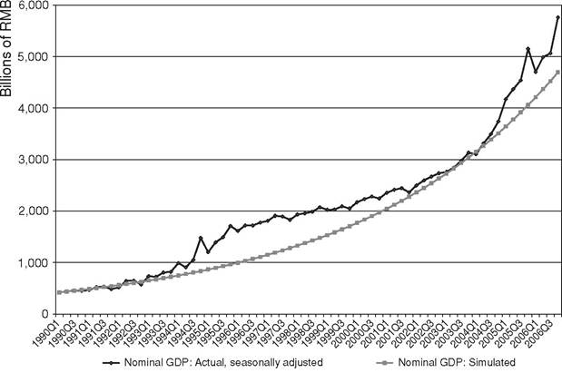
Figure 4.2. Actual vs. Simulated Values of Nominal Output, 1990-2006.
In our analysis, the unobservable target nominal GDP growth is modeled based on the trend properties of the raw data, which is not only required by the absence of a consistent series of official target values but also in keeping with the long-standing Friedmanite rationale for linking money growth to trend growth in output.
A quarterly 3.75% growth rate, with a stochastic component around this growth rate, appears to best capture the underlying properties of the data (as detailed in Burdekin and Siklos, 2008). The resulting series, together with actual GDP, is plotted in Figure 2. The results of implementing equation (1) in the original form specified by McCallum are included in Burdekin and Siklos (2008). Relative to the indicated McCallum rule, monetary policy was found to be too loose until about 1996 since actual M2 growth and monetary base growth far exceeded predicted money growth. This indicated period of monetary excess naturally coincides quite closely with the 1993-1994 inflation spike discussed in Chapter 3. With regard to the post-1996 experience, the basic McCallum rule implied that M2 growth tended to be too tight but monetary base growth, on the other hand, remained more or less in line with the rule’s predictions.In reapplying the McCallum rule to an extended 1990-2006 dataset, the estimates reported in this chapter not only allow the response to the nominal GDP output gap to be determined by the data but also simultaneously allow for money supply reactions to the rate ofchange of foreign exchange reserves,
Table 4.3. Money supply reactions based on extended McCallum Rule Estimates, 1990-2006
| Right-hand-side Variables | Ordinary Least Squares (OLS) Estimates | Generalized Method of Moments (GMM) Estimates | ||
| M2 Growth | Monetary Base Growth | M2 Growth | Monetary Base Growth | |
| Constant | 6.55 | 5.78 | 6.43 | 5.69 |
| (0.50)*** | (0.59)*** | (0.28)*** | (0.32)*** | |
| Nominal output gap | —0.02 | —0.01 | —0.04 | —0.02 |
| (0.03) | (0.04) | (0.02)a | (0.03) | |
| Post-Asian financial | —2.74 | —3.42 | —2.55 | —2.87 |
| crisis dummy | (0.66)*** | (0.79)*** | (0.37)*** | (0.42)*** |
| Rate of change of foreign | —0.07 | —0.01 | —0.05 | —0.01 |
| exchange reserves | (0.04)* | (0.05) | (0.02)** | (0.03) |
| Rate of change of the real | — 1.38 | —3.47 | —2.08 | —4.17 |
| exchange rate | (1.43) | (1.69)** | (1.05)* | (0.89)*** |
| R2 overall goodness of fit | 0.38 | 0.37 | 0.37 | 0.36 |
| J-test for over-identifying | - | - | 6.24 | 8.15 |
| restrictions | (p = 0.86)b | (p = 0.61)b | ||
Notes: Standard errors are reported beneath the coefficients; ***, **, and * indicate significance at the 99%, 95%, and 90% confidence levels, respectively.
a Denotes significance at the 89.5% confidence level.
b Denotes the exact significance level for the J-test statistic - with the insignificant values implying that the over-identifying restrictions required for the GMM estimation could not be rejected (see text under equation (2) for the list of instruments).
the rate of change of the real exchange rate, and a post-Asian financial crisis dummy set equal to one after 1997. The estimation period is from the second quarter of 1991 through the second quarter of2006. Table 4.3 reports a series of regressions of the form:
and all other variables are as previously defined.
Ordinary least squares (OLS) estimates are reported first. These estimates may not accurately reflect the People’s Bank of China’s true reaction to the
right-hand-side variables in equation (2), however, as OLS estimation comingles the central bank’s policy response with more general economy-wide reactions. This is due to the endogeneity, or non-predetermined nature, of the right-hand-side variables. Hence, the final two column of Table 4.3 show the results of reestimation using the Generalized Method of Moments (GMM) procedure to correct for this endogeneity issue. The constant, postAsian financial crisis dummy, two lags of each of the variables in the equation, and two lags of export growth were used as instruments to apply the GMM procedure.[68]
The 0.5 coefficient value for β 1 hypothesized by McCallum (1988) is not supported in the Chinese case, and the GDP gap is generally statistically insignificant - in the one case where it is marginally significant, the negative sign actually implies an accommodative, procyclical response to nominal output movements.[69] The post-Asian financial crisis dummy is negative and highly significant for both M2 and the monetary base across each of the two estimation procedures.
Monetary policy may well have remained tighter after 1997 in the face of pressures arising, first, from the need to support the exchange rate in the immediate aftermath of the Asian financial crisis, and, second, the need to offset incipient inflationary pressures arising from the reserve buildup later on. There is also some evidence of a tendency for M2 growth to slow as foreign exchange reserve growth accelerates, although this effect is neither very strong nor very highly significant. Meanwhile, the fact that the monetary base shows no significant reaction to reserve growth remains consistent with People’s Bank success in sterilizing reserve inflows.Insulating the overall level of the monetary base from the effects of reserve inflows requires that the domestic component of the base be reduced, on a one-to-one basis, when the foreign component is forced up by new reserve accumulation. Complete, or near-complete sterilization, as discerned by both He et al. (2005) and Ouyang, Rajan, and Willett (2007), implies the overall monetary base remaining invariant to increased reserve inflows,
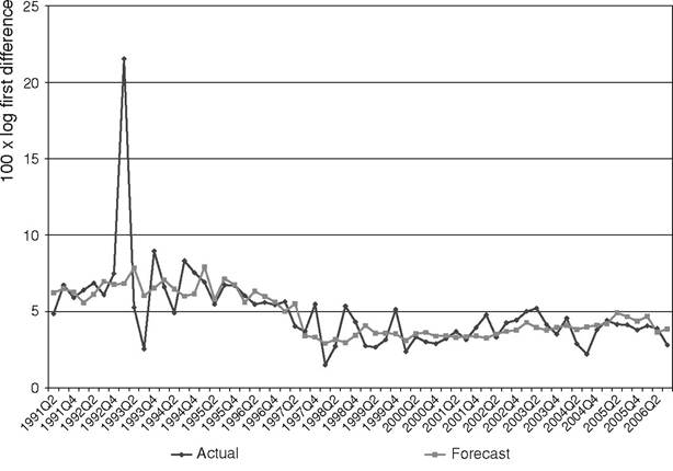
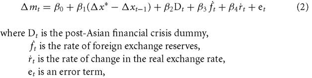
Figure 4.3. Actual vs. Fitted M2 Growth Rates Based on GMM Estimation.
therefore, consistent with the present findings.[70] On the other hand, failure to fully sterilize reserve inflows should be associated with a positive monetary base reaction to higher rates of reserve accumulation. Finally, there is evidence of a negative reaction to the real exchange rate in three cases out of four, indicating a countercyclical (stabilizing) response to real exchange rate appreciation. Real exchange rate appreciation, as experienced during much of the 1990s (Chapter 1), can arise when Chinese prices are rising faster than prices abroad. Tighter monetary policy that reduced Chinese inflation rates would tend to offset such real exchange rate appreciation.
Our final exercise is to compare the predicted values from the regressions reported in Table 4.3 to actual money growth rates observed over the 1991— 2006 period.
Given that forecast values from the alternative OLS and GMM regressions for both M2 and the monetary base proved to share almost identical trends, Figures 4.3 and 4.4 simply compare M2 and monetary base fitted values from the GMM estimation to the actual money growth rates. Figure 4.3 points to M2 being, as one would have suspected, generally too
Figure 4.4. Actual vs. Fitted Monetary Base Growth Rates Based on GMM Estimation.
loose during the 1993-1995 inflation spike - but otherwise shows actual M2 growth according quite well with the forecast values implied by the extended McCallum policy rule. Meanwhile, Figure 4.4 suggests a more moderate, but also more extended, tendency for overly high growth rates for the monetary base during 1993-1998. After that, monetary base growth looks to have become too tight in 1998-1999, at the time that the Chinese economy entered deflation, but subsequently follows a similar trend to the forecast values. Overall, the strong suggestion of overly loose policy in the early to mid-1990s followed by indications (from the performance of monetary base growth) of overly tight policy at the end of the 1990s seems quite consistent with actual experience. It is also interesting to see that sustained deviations from forecast values were generally avoided after 2000 in spite of the pressures arising from record rates of foreign reserve accumulation and the claimed undervaluation of the renminbi.
More on the topic Estimation Results:
- Estimation Results
- Summary of Empirical Results
- In this section, we will present the results of the execution of the simulation using the model described in the previous section.
- Variations on the Nelson-Phelps model
- RESULTS AND ANALYSES
- Model prediction
- Chapter 5 Determinants of Banking Profitability in Portugal and Spain: Evidence with Panel Data
- The Macroeconomic Model
- The Netherlands and the UK: The Witteveen Reports and their contradictory results
- Section 6 Emerging Trends