Growth without Scale Effects

The models used so far feature a scale effect in the sense that a larger population, L, translates into a higher interest rate and a higher growth rate. This is problematic for three reasons as argued in a series of papers by Chad Jones and others:

(1) Larger countries do not necessarily grow faster (though the larger market of the United States or European economies may have been an advantage during the early phases of the industrialization process; see also Chapter 21).

(2) The population of most nations has not been constant. With population growth as in the standard neoclassical growth model, e.g., L (t) = exp (nt) L (0), these models would not feature balanced growth, rather, the growth rate of the economy would steadily increase over time and output per capita would reach infinity in finite time (“explode”).

(3) In the data, the total amount of resources devoted to R&D appears to increase steadily, but there is no associated increase in the aggregate growth rate.

Each one of these arguments against scale effects can be debated (for example, by arguing that countries do not provide the right level of analysis because of international trade linkages or that the growth rate of the world economy has indeed increased when we look at the past 2000 years rather than the past 100 years). Nevertheless together they do suggest that the strong form of scale effects embedded in the baseline endogenous technological change models may not provide a good approximation to reality. These observations have motivated Jones (1995) to suggest a modified version of the baseline endogenous technological progress model. While the type of modification to remove scale effect can be formulated in the lab-equipment model (see Exercise 13.21), it is conceptually simpler to do so in the context of the model with knowledge spillovers discussed in the previous section.

More specifically, consider the model of the previous section with only two differences. First, there is population growth at the constant exponential rate n, so that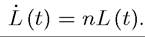

The economy admits a representative household, which is also growing at the rate n, so that its preferences can be represented by the standard CRRA form:

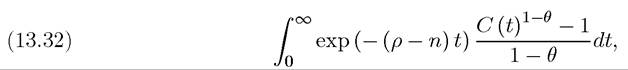
where C (t) is consumption of the final good of the economy at time t, which is produced as before (with the production function (13.2)).

Second, in contrast to the knowledge-spillovers model studied in the previous section, the R&D sector only admits limited knowledge spillovers and (13.24) is replaced by

where φ < 1 and Lr (t) is labor allocated to R&D activities at time t. Labor market clearing requires

(13.34) Le (t) + Lr (t) = L (t),

where Le (t) is the level of employment in the final good sector and L (t) is population at time t.

The key assumption for the model is that φ < 1. The case where φ = 1 is the one analyzed in the previous section, and as commented above, with population growth this would lead to an exploding path, leading to infinite utility. However, the model is well behaved when φ < 1.

Aggregate output and profits are given by (13.25) and (13.26) as in the previous section. An equilibrium is also defined similarly. Let us focus on the BGP, where a constant fraction of workers are allocated to R&D, and the interest rate and the growth rate are constant. Suppose that this BGP involves positive growth, so that the free-entry condition holds as equality. Then, the BGP free-entry condition can be written as (see Exercise 13.18):

As before, the equilibrium wage is determined by the production side, (13.13), as w (t) = βN (t) / (1 — β). Combining this with the previous equation gives the following free-entry condition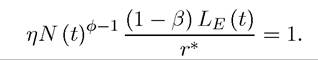

Now differentiating this condition with respect to time:

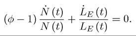
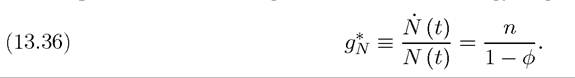
Since in BGP, the fraction of workers allocated to research is constant,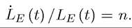 This implies that the BGP growth rate of technology is given by

From eq.

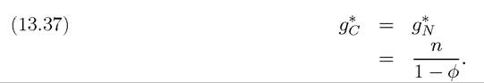
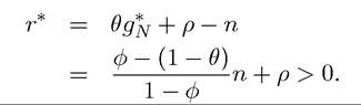
The consumer Euler equation, equivalent of (11.4) incorporating the fact that the discount factor is ρ — n instead of ρ, then determines the BGP interest rate as

The most noteworthy feature is that this model generates sustained and exponential growth in income per capita in the presence of population growth. More interestingly, in order to achieve this growth rate, it allocates more and more of labor to R&D. This is possible because of population growth. The reason for this is that the technology for creating new ideas, (13.33), only features limited spillovers, thus to maintain sustained growth, more resources need to be allocated to R&D.

Proposition 13.5. In the above-described expanding input-variety model with limited knowledge spillovers as given by (13.33), starting from any initial level of technology stock N (0) > 0, there exists a unique BGP in which, technology and consumption per capita grow at the rate as given by (13.36), and output grows at rate

495

This analysis therefore shows that sustained equilibrium growth of per capita income is possible in an economy with growing population. Intuitively, instead of the linear (propor­tional) spillovers in the baseline Romer model, the current model allows only a limited amount of spillovers. Without population growth, these spillovers would affect the level of output, but would not be sufficient to sustain long-run growth.

It is also worth noting that these models are sometimes referred to as “semi-endogenous growth” models, because while they exhibit sustained growth, the per capita growth rate of the economy, (13.37), is determined only by population growth and technology, and does not respond to taxes or other policies. Some papers in the literature have developed models of endogenous growth without scale effects, with equilibrium growth responding to policies, though this normally requires a combination of restrictive assumptions.

13.4.