KEY DIAGRAM 7

The aggregate demand-aggregate supply model

The AD-AS model shows the determination of the price level and output. In the short run, before prices adjust, equilib­rium occurs at the inter­section of the AD and SRAS curves.

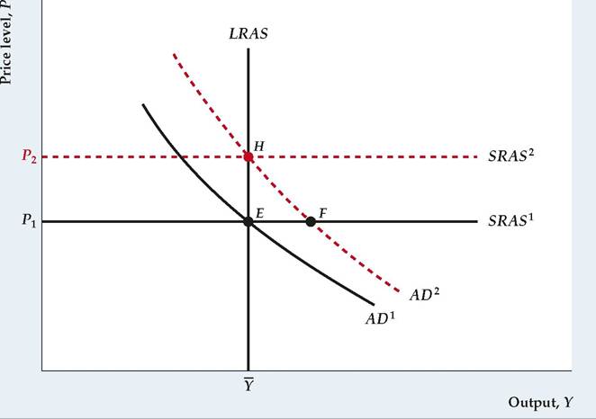
Diagram Elements

■ The price level, P, is on the vertical axis, and the level of output, Y, is on the horizontal axis.

■ The aggregate demand (AD) curve shows the aggre­gate quantity of output demanded at each price level. The aggregate amount of output demanded is deter­mined by the intersection of the IS and LM curves (see Fig. 9.10). An increase in the price level, P, reduces the real money supply, shifting the LM curve up and to the left, and reduces the aggregate quantity of output demanded. Thus the AD curve slopes downward.

■ The aggregate supply curves show the relationship between the price level and the aggregate quantity of output supplied in the short run and in the long run. In the short run, the price level is fixed, and firms supply whatever level of output is demanded. Thus the short-run aggregate supply (SRAS) curve is hori­zontal. In the long run, firms produce the amount of output that maximizes their profits, which is the full­employment level of output, Y._Because aggregate output in the long run equals Y regardless of the price level, P, the long-run aggregate supply (LRAS) curve is a vertical line at Y = Y.

Factors That Shift the Curves

■ The aggregate quantity of output demanded is deter­mined by the intersection of the IS and the LM curves. At a constant price level, any factor that shifts the IS-LM intersection to the right increases the aggre­gate quantity of goods demanded and thus also shifts the AD curve up and to the right. Factors that shift the AD curve are listed in Summary table 14.

■ Any factor, such as an increase in the costs of produc­tion, that leads firms to increase prices in the short-run will shift the short-run aggregate supply (SRAS) curve up. Any factor that increases the full-employment level of output, Y, shifts the long-run aggregate sup­ply (LRAS) curve to the right. Factors that increase Y are listed in Summary table 11.

Analysis

■ The economy's short-run equilibrium is represented by the intersection of the AD and SRAS curves, as at point E. The long-run equilibrium of the economy is represented by the intersection of the AD curve and LRAS curve, also at point E. In the long run, output equals its full-employment level, Y.

■ The short-run equilibrium can temporarily differ from the long-run equilibrium as a result of shocks or pol­icy changes that affect the economy. For instance, an increase in the nominal money supply shifts the aggregate demand curve up and to the right from AD^[160] to AD ^[161]. The new short-run equilibrium is repre­sented by point F, where output is higher than its full­employment level, Y. At point F, firms produce an amount of output that is greater than the profit­maximizing level, and they begin to increase prices. In the new long-run equilibrium at point H, output is at its full-employment level and the price level is higher than its initial value, P₁. Because the new price level is P₂, the short-run aggregate supply curve shifts up to SRAS ², which is a horizontal line at P = P₂.

►