Interspecific competition in a food web context

The focus on competitive coexistence in the ecological literature would lead one to believe that competing species have the greatest effect on whether a species can per­sist. The important part of the word ‘coexistence’ is ‘existence’.

A question related to existence is how those species at other trophic levels affect the competitive interactions between species on a particular trophic level. Should predators on a higher level be regarded as a force that reduces or eliminates com­petitive effects on abundances? These questions are discussed briefly below. Not surprisingly, the answer depends on the measure of competition that is chosen. The model explored below is arguably the simplest possible one in which the effects of competition in a food web can be explored. Nevertheless, it is not simple.

The 6-species model used here has two species on each of the three trophic levels. A similar model was used by Abrams (1993) to assess the generality of top-down and bottom-up effects in food webs. This model was also used by Matsuda and Abrams (2006) to evaluate optimal harvesting strategies for exploiting fish communities. In this food web, the two species on the middle level (‘consumers') interact indirectly both via the predators at the top trophic level and the resources at the lowest level. The resources are assumed to be biotic. The equations given below in Box 7.1 have type II functional responses for consumer species and include intraspecific density dependence for the predator species.

The simplest version of this model is one in which all handling times are zero and there is no direct intraspecific interference on the top trophic level (i.e., all Y values are zero). This produces a ‘MacArthur' model. The interactions at each troph­ic level can be characterized by the response of each species to a small change in the per capita mortality rate of the other species at that trophic level. (Of course, this is not a complete description of the variety of possible responses to a larger range of perturbation parameters and magnitudes.) The starting conditions in the

Box 7.1 Competition in a simple 6-species, 3-trophic level model

The full model used here has the following form:

The parameters in the above equations have the meanings given in similar equations in previous chapters. The resource density dependence parameter, k, has been given dual sub­scripts to distinguish intraspecific (k_ii) from interspecific (kj) effects on each species i. The double subscripts involving N or P parameters give the identifier for the consumer/predator first and resource/prey second. The parameters Y_ij are the ‘interference' coefficients of the predator, and the first subscript gives the affected species and the second gives the effector. The presence of interference has dynamic consequences that are in some ways similar to those produced by an additional (higher) trophic level.

present simple example assume that the two species at each of the top two lev­els are equivalent to each other except for their consumption rates of resources. The two species on the mid and top level are also characterized by having mirror image consumption rates of their two prey species.

The interactions at each level in the simple MacArthur style version of the model (no handling time or predator interference) are as follows:

1. The response of each of the top-level species to mortality in the other top-level species can be positive or negative. If there is no interspecific competition on the lowest level (k_ij = 0 for i =j, meaning α = 0), the results of Levine (1976) apply to the top and middle levels. This means that the top consumers have mutually positive effects when resource overlap of the mid-level species is greater than resource over­lap of the top-level species (i.e., c is closer to 1/2 than is C). If competition between the two bottom-level species were allowed, high enough competition could reverse the sign of the interaction between top-level species.

2. Ifthe top two levels have equivalent prey partitioning (C = c), then there is no com­petition between the species on the top level, unless the resources compete with each other. With some between-resource competition, given C = c, the between- predator effect is again negative (P_i increases with Dj), and the magnitude of the positive effect of Dj on P_i increases as the level of between-resource competition increases (again provided that all species persist).

3. The second level (N₁, N₂) has no interaction based on response to a small change in the per capita mortality of the other species at that level, and this does not depend on any parameter, so long as all six species persist. (Recall the assumption of no interference competition (Y_ij = 0) in either top-level species.) The equilib­rium abundances of the two mid-level species are completely determined by the characteristics of the two species on the top level (provided that all six species persist).

4. The bottom-level species (R₁, R₂) respond to changes in each other’s neutral parameter r as though the higher-level species were absent. They have zero effect on each other unless they compete directly with each other (α >0; i.e., k_ij > 0). This is because the equilibrium abundances of their consumers (the mid-level species) are controlled by the top-level species, eliminating the apparent competition that would otherwise occur. This is again true only so long as all species persist.

In summary, if all three levels share resources in this simple case of a MacArthur style model, the bottom-level species are the only ones for which mutually negative effects on equilibrium abundance revealed by a neutral perturbation can be assumed when there is ‘direct’ competition between them (α > 0). The middle level has no interaction between its two species based on their lack of change in response to a small shift in a neutral parameter of the other species. This result for the middle level remains true for nonlinear functional responses of the top predators, provided that the equilibrium point is stable, and the predators are solely limited by their food con­sumption rate (i.e., the Ó parameters are zero). When the bottom resources do not interact, the interaction between the top-level species is determined by whether the top-level predators are more generalized than the mid-level predators; i.e., C is closer to 1/2 than is c (negative effects) or C is further from 1/2 than c (positive effects).

The effect of a large magnitude change in the mortality rate of one intermediate (consumer) species can be extinction. This result is inevitable if the mortality rate of one consumer is increased sufficiently. The disappearance of one of the mid-level species will generally also entail extinction of one of the top predators in the absence of strong interference at the top level. Extinction of a top predator may also pre­cede extinction of the second consumer. A sufficient decrease in the mortality rate of one competitor will always produce extinction of the other competitor in a 2-species Lotka-Volterra system. However, that is not the case here. Relatively low produc­tivity systems (low r values) are required for extinction to be the consequence of a low enough mortality rate of the superior consumer on the intermediate trophic level. Once this occurs, coexistence of the top two consumers becomes impossible unless one or both have interference coefficients (Y_ii > 0). When the Ó coefficient of the remaining consumer is zero, then the abundance of the mid-level consumer again becomes independent of its own per capita death rate. Increases in its death rate simply reduce the equilibrium of the remaining top consumer.

The full model in Box 7.1 allows type II responses and direct density dependence of top-consumer death rates. These often alter the results for the simple case described above. Type II responses on the top level do not change the independence of mid­level equilibrium abundances on the parameters of lower-level species, and on the mortality rates of the mid-level species themselves. However, type II responses, even when they do not produce population cycles, alter the interaction of the top-level species. It is no longer true that these species do not interact in a symmetrical system with equal partitioning on the top two levels (C = c) and no competition between resources.

If the handling time produces population cycles, the mean population sizes usually respond differently to parameter changes than do the equilibrium population sizes. Independent of the handling time, self-limitation on the top trophic level also can cause differences in the signs of responses to parameter change. If the self-limitation terms (Y_ij) are non-zero, this means that equilibrium abundances of the middle level will be influenced by their consumption rates of the bottom-level species, and by other lower level parameters. Each mid-level species’ abundance is also affected by mortali­ty in the other mid-level species. However, these effects are likely to be relatively small if the top-level species’ interference parameters (Y) are themselves small.

A comprehensive analysis of the cases with both handling time and self-limitation has not been carried out. Two related examples with handling time and the poten­tial for cycles are provided here, simply as an illustration of the large range of effects that may occur. Both are cases in which the top two trophic levels consist of two species with ‘mirror image' consumption rates of their two prey. As a result, the equilibrium has equal abundances of the two species at each level. The two exam­ples both assume identical partitioning for the two top levels. Equal partitioning in the corresponding model with no handling time, no top predator interference, and no interspecific resource competition, would imply no competitive effect of a small change in mortality for either of the species on each of the top two levels.

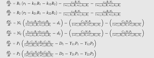
Figure 7.2 shows the population dynamics of the four species on the top two trophic levels in an example that can exhibit anti-synchronized dynamics. The mean abundances of the two species on a given level are the same for all three levels. There is an alternative attractor for this system (not illustrated) with much smaller ampli­tude and perfectly synchronized cycles. Starting at the anti-synchronized attractor shown in Figure 7.2, a 10% increase (d₂ = 0.275) in the mortality rate of one the mid-level consumers (which has no effect on the equilibrium abundances of either of the mid-level species) produces small decreases in the mean abundances of both mid-level consumers (with a larger decrease for the species suffering increased mor­tality). This mid-level mortality perturbation produces much larger changes in the abundances of the top-level species, with the top predator more specialized on the perturbed prey decreasing by a relatively large amount, while the other predator increases by a somewhat smaller amount. Both changes are much greater in mag­nitude than those of the second-level species. If mid-level mortality d₂ is increased to 0.3, the system becomes stable, and the abundances of the two intermediate predators equalize. Further increases in d₂ do not alter these abundances until d₂ is sufficient to cause extinction of top predator 2 at approximately d₂ = 0.46. This causes the system to undergo limit cycles, and it also causes a large increase in the mean abundance of top predator 1 (to 0.6289), a large decrease in the mean abundance of intermediate predator 2 (to 0.1084), and a modest increase in the mean abundance of intermediate predator 1 (to 0.2178). A slight further increase in d₂ to 0.47 results in the extinction of intermediate predator 2 from all initial conditions, producing a system with cyclic dynamics of top predator 1, intermediate predator 1, and the two resources.

Figure 7.3 shows the dynamics of the top two trophic levels for a second example with symmetrical attack rate values and the same relative specialization for both the top two levels (as in the preceding figure). Here, the handling times for the top-level predators are increased to Hj = 1.5 and the initial death rates of species at that level are decreased D₁ = D₂ = 0.05 (and the other parameters are identical to those of Fig­ure 7.2; in particular d₁ = d₂ = 0.25 in the initial symmetrical condition). This set of parameters produces quasi-periodic cycles, which makes it difficult to obtain precise measures of the mean values. However, the effect of a small increase in the mortality rate of one of the intermediate predators again decreases the mean abundance of both predators by small amounts, while having larger effects (one positive, one negative) on the abundances of the top predators. In this case increasing d₂ never stabilizes the equilibrium, although the cycles become simpler inform when d₂ is sufficiently large.

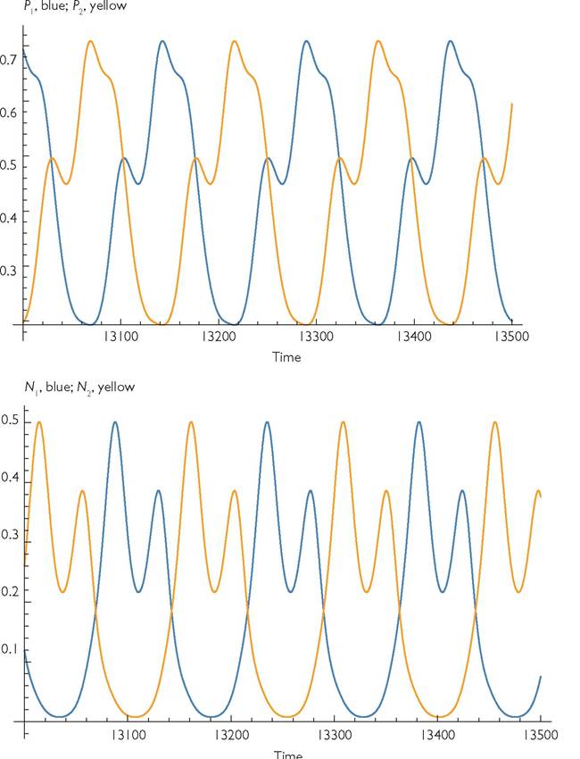
Fig. 7.2 Dynamics of the top two trophic levels for the model given in Box 7.1. The consumers have ‘mirror image' consumption rates of the two resources they consume. The parameter values are: r₁ = r₂ = 1; k₁₁ = k₂₂ = 1; k₁₂ = k₂₁ = 0, b_ij = 1; c₁₁ = c₂₂ = 0.7; C12 = C21 = 0.3; d1 = d2 = 0.25; B_ij = 0.5; C_n = C22 = 0.7; C12 = C21 = 0.3; H_ij = 1.25; D1 = D2 = 0.075; Yj = 0.

Fig. 7.3 Dynamics of the top two trophic levels for the model given in Box 7.1. Most of the parameters are identical to those given in Figure 7.2. 'The parameters that differ are; H_ij = 1.5, and D₁= D₂ = 0.05. These changes alter the nature of the population cycles and increase their amplitude.

The mortality on the intermediate predator 2 (d₂) primarily reduces the mean density of top predator, P₂, and only causes small changes in the mean abundances of N ₁ and N₂. However, an increase in d₂ increases the mean abundance of N₁, indicating a neg­ative effect of mid-level species 2 on species 1. When d₂ is raised to 0.46, the ratio of the mean P₁ to the mean P₂ becomes 114.26, while the corresponding ratio of mean N₁ to mean N₂ is 1.2205. This again reflects the much larger effect on predators than on the one competitor of this mid-level species. When d₂ = 0.47, top predator species 2 goes extinct and the ratio of mean densities of N₁ relative to N₂ grows to 5.893. At d₂ = 0.48, N₂ also goes extinct. In the six-species system with all species present, the impact of a mid-level predator’s mortality on the abundances of the higher-level species is much greater than its impact on its competitor. The effect on the competitor is only non-zero in cycling systems, or in the presence of interference terms on the top level.

Another question that can be addressed with the model in Box 7.1 is how the per­sistence of a given species is impacted by another species on the same trophic level vs those on other trophic levels. This is central to the issue of whether existence of a giv­en species is more sensitive to changes in a competitor, a predator, or a food species. It also bears on the question of whether direct effects measured by changes in equilib­rium abundance are needed to produce indirect effects. All these questions are raised by the phenomenon described above—i.e., the fact that the two middle-level species do not affect each other’s abundance when ‘effect’ is measured by the sensitivity to a small change in a neutral parameter of the other species. In spite of the lack of a measured effect on their own population sizes, the two mid-level species transmit an effect of a mortality change in either of the top predator species to the bottom-level resources. Thus, increasing top predator 1’s mortality D₁ will usually affect both of the lower-level resources, and at least one of those resources will increase.

Of course, the above is one of the simplest possible food web models that includes competition and more than two trophic levels. Even here, I have only discussed some highly simplified or highly symmetrical cases.

7.6